Syllabus Map

Study map: Syllabus Study Map

Overview

Ensemble methods in machine learning combine multiple individual models (weak learners) to create a single more accurate predictive model.
This usually works as it averages out individual model errors.
Ensemble methods are typically used when data is:
- Noisy,
- Complex or
- Very diverse

Motivation for Ensemble Learning

Why Single Models Fail

Single models are prone to inaccuracies on diverse data, including issues like:
- Overfitting
- Underfitting
- Sensitivity to noise
- Sensitivity to data splits

Error Decomposition

Prediction Error measures how far model predictions are from the true labels.
Generalisation Error measures the expected Error on unseen data.
Total expected Error can be decomposed to Bias² + Variance + Irreducible Noise.
- Bias: Underfitting due to simplistic assumptions.
- Variance: Overfitting due to hypersensitivity to data.
- Irreducible noise: Randomness in data.
Ensemble methods solve this by :
- Averaging multiple models to reduce variance.
- Sequential correction to reduce bias.
- Improving model diversity to reduce correlated errors.

General Ensemble Framework

Base Learners

Weak learners are simple models that have low complexity and accuracy on their own.
Examples of these include:
- Decision Trees
- Linear Models
- k-Nearest Neighbours
Ensembles tend to yield better results when there is a significant diversity among the models.
Random algorithms (like random decision trees) can be used to produce a stronger ensemble than very deliberate algorithms (like entropy-reducing decision trees).

Combining Predictions

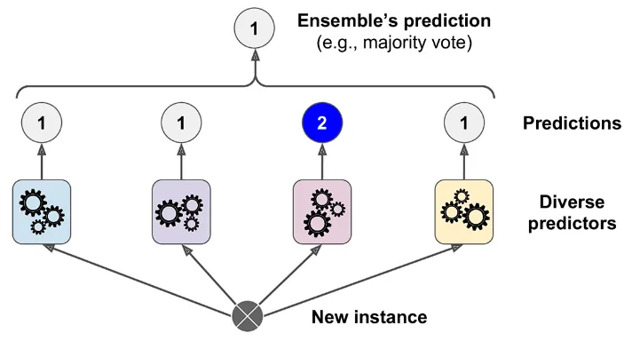
After collectivising these weak learners, we have to combine their predictions in a meaningful way to improve the model’s combined performance.
This can be done through:
- Majority voting: Consensus of models to decide on the class label
- Weighted voting: Best choice of class label based on the significance of each model
- Averaging: Obtaining the mean of results for a continuous value
- Probability Aggregation: Best result based on the confidence of each model

Bagging (Bootstrap Aggregation) and Pasting

Core Idea

Bagging uses the same training algorithm for every predictor.
However, it trains them on different random subsets of the training set.
When sampling is performed with replacement, this method is called bagging.
When sampling is performed without replacement, it is called pasting.

Why Bagging Works

Each individual learner has a lower variance than if it were trained on the entire dataset.
Aggregation thus allows the ensemble to improve variance by making averaging random errors and prevent overfitting.
This in turn helps models be more stable by reducing sensitivity to noisy training data.

Algorithm Outline

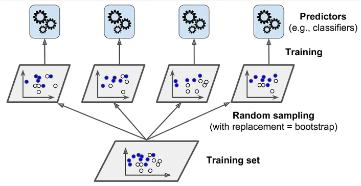
A training set is split into random subsets for training.
Weak learners are trained using these random subsets of data.
A prediction for a new instance is made by simply aggregating the predictions of all predictors.
- For classifiers, this is done by the statistical mode.
- For regressors, this is done by the statistical mean.

Out-of-Bag Evaluation

With bagging, some instances may be sampled several times , while others may not be sampled at all.
By obtaining the out-of-bag dataset, an estimate of model performance on unseen training data, which should be comparable to the test set

Random Patching and Random Subspaces

Random Subspaces

Each model is trained on all data points, but they can only see a random subset of features.
This prevents dominance of features in affecting performance.

Random Patching

Combines both:
- Random sampling of data points
- Random sampling of features
Each model sees a different subset of samples and features.

Random Forests

Motivation

Bagging does not adequately address the issue of correlation between trees.
When datasets have strong features, the decision trees will choose those features as top-level splits.
This results in highly correlated trees, which diminishes the variance-decreasing ability of bagging.
This causes overfitting and worse model performance for deep trees

Core Principles

Random Forests combines both:
- Random sampling of data points
- Random sampling of features
Each model sees a different subset of samples and features.

Algorithm Overview

For each tree in the forest, a random subset of the original training data is selected with replacement.
At each node during the tree-building process, only a random subset of features is considered for the best split.
A decision tree is grown on each unique data and feature subset until a stopping criterion.
A prediction for a new instance is made by simply aggregating the predictions of all predictors.
- For classifiers, this is done by the statistical mode.
- For regressors, this is done by the statistical mean.

Extra-Trees

Building on the random forest algorithm, it is possible to make trees even more random
This is done by using random thresholds for each feature rather than searching for the best possible thresholds
Refer to the Decision Tree notes to learn more about the node structure.
This trades more bias for a lower variance in the models.

Boosting

Core Idea

Boosting focuses on sequential learning, where multiple weak models are trained one after another to form a strong model.
Each model tries to correct for the errors of the predecessors by adjusting weights of the samples.

Why Boosting Works

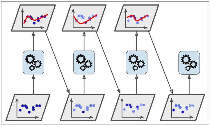
Boosting reduces bias by correcting for errors from previous iterations of the model.
This also builds complex decision boundaries through additive modelling.

AdaBoost

Key Concepts

AdaBoost works by paying more attention to the training instances that the predecessor misclassified.
This results in new predictors focusing more and more on hard cases in the samples.

Algorithm Outline

Initialise equal sample weights and train a first weak classifier.
Compute the classifier’s weighted error and assign it a model weight.
Increase weights of misclassified samples, decrease weights of correctly classified samples, then normalise.
Train the next weak classifier on the reweighted data and repeat steps 2-3 for multiple rounds.
Make the final prediction using a weighted majority vote of all weak classifiers.

Intuition

Mistakes made by predecessor models get more attention (higher weight) while retraining.
This means that the model can progressively correct its mistakes.
However, this makes it sensitive to noisy labels and outliers.

In-Depth Algorithm

Step 1: Instantiation and Setting Weights

Each instance weight $w_i$ is set to $1/m$ .
The model is trained on the samples.

Step 2: Calculate Weighted Error Rate

The weighted Error rate $r_j$ is computed on the training set for model $j$ .

r_j = \frac{\sum^{m}_{i=1} w_i \space \text{ s.t. } \hat{y}_{i,j} \ne y_i}{\sum^{m}_{i=1} w_i}

Step 3: Calculate the Predictor’s Weight

The weight $a_j$ $a_{j}$ of the predictor $j$ $j$ will be calculated to assess its performance.
- The more accurate the predictor is, the higher its weight will be.
- If it is just guessing randomly, then its weight will be close to zero.
- However, if it is most often wrong, then its weight will be negative.

\alpha_j = \frac{1}{2} \eta \log \frac{1 - r_j}{r_j}

Step 4: Update the Weights of the Samples

The instance weights of the misclassified instances are boosted for predictor $j$ .

w_i \begin{cases} w_i \exp(-\alpha_j) \quad \text{if } \hat y_i = y_i \\ w_i \exp(\alpha_j) \space \space \space \quad \text{if } \hat y_i \ne y_i \end{cases} \forall i \in \{1, 2, 3, ..., m\}

The new weights are normalised.

w_i \leftarrow \frac{w_i}{\sum^{m}_{i=1}w_i} \forall i \in \{1, 2, 3, ..., m\}

Step 5: Make Predictions

AdaBoost computes the predictions of all the predictors and weighs them using the predictor weights $\alpha_j$ .

\hat y = \argmax_k \sum^{N}_{j=1, \space \hat y_j = k} \alpha_j

Gradient Boosting

Core Idea

Like AdaBoost, Gradient Boosting works by sequentially adding predictors to correct its predecessors.
However, it fits each new predictor to the residual errors (loss) of the current model.

Algorithm Outline

Initialise the model with a constant prediction that minimises the loss.
Compute the negative gradient (residuals) of the loss with respect to the current predictions.
Fit a new weak learner to these residuals.
Scale the learner by a step size and add it to the ensemble.
Repeat steps 2–4 for the desired number of iterations.

Loss Functions

Mean Squared Error loss for regressors.
Negative Log-Likelihood for classifiers.

How XGBoost Handles Missing Values

XGBoost handles missing values natively, so you usually do not need separate imputation.
During training, for each split, it learns a default direction (left or right) for samples with missing feature values.
It chooses the default direction that gives the best gain in the objective.
During inference, if a feature value is missing, the sample follows that learned default branch.
This lets XGBoost treat missingness as potentially informative rather than only as missing data noise.

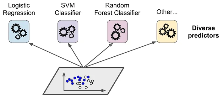
Stacking

Core Idea

Stacking is an ensemble method that uses meta-learning.
Instead of simple averaging or voting, it trains a meta-model to combine base model predictions.
The meta-model learns how to weight and combine different models optimally.
Works best when base models are very different (high diversity).

Architecture

Base learners (Level-0 models):
- Different algorithms (e.g. trees, SVMs, kNN, linear models).
- Each trained on the original dataset.
- Each outputs predictions.
Meta-model (Level-1 model):
- Takes predictions of base learners as input features.
- Learns how to combine them.
- Produces final prediction.
Often uses cross-validation to avoid data leakage.

Why Stacking Works

Different models capture different patterns in the data.
Some models perform better in certain regions of the feature space.
The meta-model learns:
- Which models to trust more
- Under what conditions
Can reduce both bias and variance.
More flexible than bagging or boosting.

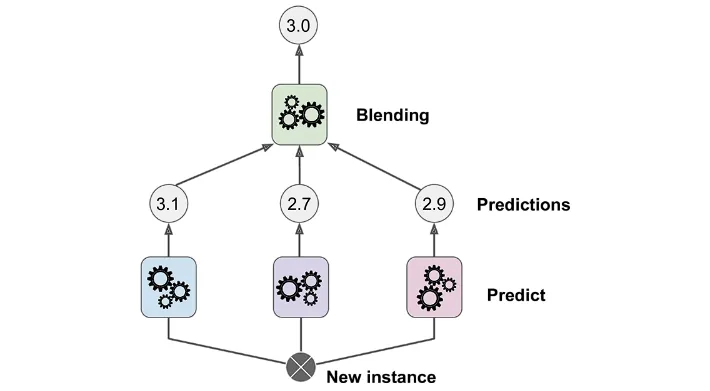
Blending vs Stacking

Both combine multiple base learners using a meta-model.
Main difference lies in how the meta-model is trained.

Blending

Uses a hold-out validation set.
Base models are trained on training set.
Meta-model is trained on predictions from validation set.
Simpler, but wastes data.

Stacking

Uses cross-validation.
Base models generate out-of-fold predictions.
Meta-model is trained on all data.
More data-efficient but more complex.

Bias–Variance Tradeoff in Ensembles

How Bagging Affects Bias & Variance

Bagging mainly reduces variance.
Each model overfits differently.
Averaging predictions cancels out noise.
Does not significantly reduce bias.
Works best for:
- High-variance models (e.g. decision trees).

How Boosting Affects Bias & Variance

Boosting mainly reduces bias.
Sequential learning allows complex patterns to be learned.
Can fit complicated decision boundaries.
However:
- Can increase variance.
- Sensitive to noisy labels and outliers.

How Stacking Affects Both

Stacking can reduce both bias and variance.
Depends heavily on:
- Choice of base models
- Choice of meta-model
If base models are diverse:
- Bias is reduced
- Variance is reduced
If base models are similar:
- Benefits are limited.

Ensemble Methods In Practice

When to Use Ensemble Methods

When single models underperform and you can afford extra compute.
When base learners have complementary Error patterns.
When variance reduction or bias reduction is a primary goal.
When you need strong performance on tabular data.

When Not to Use Ensemble Methods

When training data is very small and overfitting risk is high.
When model debugging and traceability are critical.
When you need real-time updates or streaming inference.
When deployment size and latency budgets are tight.

Practical Notes

Tuning and Diversity

Use cross-validation or out-of-bag estimates to tune ensembles.
Keep base models diverse to avoid correlated errors.

Reliability and Overfitting

Monitor calibration; averaging can still be miscalibrated.
Apply early stopping for boosting to control overfitting.