Syllabus Map

Study map: Syllabus Study Map

Introduction

Overall Goals

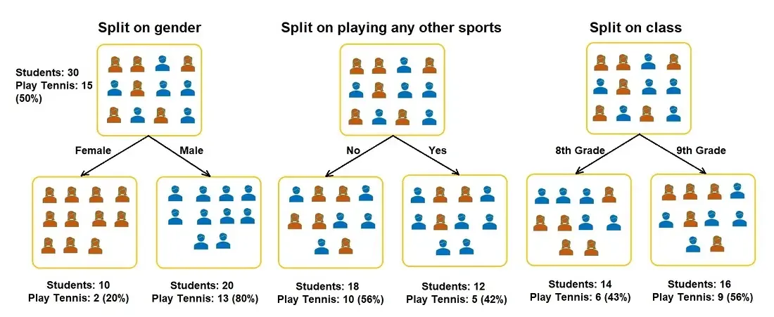
Recursively split the dataset to improve purity
Done until no further meaningful split is possible

Structure of a Decision Tree

Root Node

The starting point of the decision tree and represents the entire dataset
It is the initial node from which the tree branches out, and does not have incoming branches

Decision Node

These nodes represent a decision point based on a feature of the data
They have incoming and outgoing branches, as they split the data into sub-nodes

Leaf Node

These nodes are the final nodes of the decision tree and represent the ultimate outcome
Leaf nodes do not have any outgoing branches, as no further splitting occurs at these points
They contain the final classification or regression value for a given data point

Parent Node

This is a relative term, referring to any node that splits into two or more child nodes.

Child Node

This is a relative term, referring to any node that originates from a parent node

Training Algorithm

Step-by-Step Procedure

1. Start with the full training dataset at the root node

All samples and labels are considered together.

2. Check if the node should stop splitting

All samples belong to one class, or
The stopping condition is met.

For each feature

Evaluate all possible split points.

For numeric features:

Sort unique values.
Compute midpoints between consecutive values.
Each midpoint = potential threshold

For categorical features:

Consider subsets of categories or one-hot encodings.

3. Compute the impurity or loss for each possible split

Use Entropy / Information Gain or Gini Index (for classification).
Use Mean Squared Error (for regression).

4. Select the split with the best score

Highest information gain or lowest impurity.
Record the chosen feature and threshold.

5. Partition the dataset into child nodes

Left node → samples satisfying the condition
Right node → samples not satisfying it

7. Repeat recursively for each child node

Treat each child as a new dataset.
Apply the same splitting logic.
Stop when leaf conditions are met.

Recursive Splitting Logic

The process is greedy: it chooses the best split at each step, not globally optimal.
The resulting tree can overfit, which is why pruning is necessary.
Real implementations (like CART) use binary splits only.

Splitting Criteria

Information Gain

Information Gain is applied to quantify which feature provides maximal information about classification based on entropy
The intention is decreasing the entropy initiating from the root node to the leaf nodes.
The information gain $IG$ from splitting the set of values in a parent node $S$ is

IG(S, t) = H(S) - \frac{|S_L|}{|S|}H(S_L) - \frac{|S_R|}{|S|}H(S_R)

Where:
- $H(S)$ is entropy before splitting,
- $H(S_L), H(S_R)$ are the entropy of left and right subsets respectively,
- $|S|, |S_L|, |S_R|$ are the number of samples in the parent and child nodes respectively.

Entropy

The entropy of a random variable quantifies the average level of uncertainty with the variable’s potential states
Essentially, it is the measurement of the impurity or randomness in the data points
The entropy of a set $S$ is defined as

H(S) = - \sum_{y \space \in \space \mathcal{S}} p(y) \space \log_2 p(y)

Where:
- $y$ has the discrete states $y \in \mathcal{Y}$

GINI impurity

Calculates the probability of a feature classified incorrectly when selected randomly
If all the elements are linked with a single class then it can be called pure
The GINI impurity of a set $S$ is defined as

H(S) = 1 - \sum_{y \space \in \space \mathcal{S}} p(y)^2

Where:
- $y$ has the discrete states $y \in \mathcal{Y}$

Mean Squared Loss (MSE)

Regression-based MSE over a set $S$
The Mean Squared Error of a set $S$ is defined as

\text{MSE}(S) = \frac{1}{|S|} \sum_{(x, y_S) \in S} (y - \bar y_S)^2

Where:

$\bar y_s$ is the average value of $y$ in set $S$

\bar y_S = \frac{1}{|S|} \sum_{(x, y_s) \in S} y

Data Splitting (CART)

Feature Type	Split Condition	Split Decision	Example Condition
Numeric / Continuous	x < t or x > t	$\cdot$ Sort all unique values of (x) $\cdot$ Compute midpoints between consecutive values $\cdot$ Each midpoint = possible threshold (t)	`Age < 32.5`
Ordered Categories	rank(x) < t	$\cdot$ Map categories to ranks $\cdot$ Treat as numeric thresholds	`EducationLevel ≤ 2`
Binary Categorical	x = v	$\cdot$ Single split into {v} vs. {not v}	`IsStudent = Yes`
Multi-Categorical	x ∈ S or x ∉ S	$\cdot$ Enumerate all possible subsets S of categories $\cdot$ Often one-hot encode and treat as binary features	`Colour ∈ {Red, Blue}`
Boolean	x < 0.5 or x ≥ 0.5	$\cdot$ Treated as numeric with only one possible threshold	`IsWeekend < 0.5`

Stopping Condition

Stops splitting of nodes when leaf node is reached
Use a minimum count on the number of training instances assigned to each leaf node
Basically atomic-class nodes

Pruning Branches

Goals of Pruning

Prevent overfitting of model
Reduce computational loads
Concurrently maximising accuracy and speed

Pre-Pruning (Early Stopping)

Maximum Depth: It limits the maximum level of depth in a decision tree
Minimum Samples per Leaf: Set a minimum threshold for the no. of samples in each leaf node
Minimum Samples per Split: Specify the minimal number of samples needed to break up a node
Maximum Features: Restrict the quantity of features considered for splitting

Post-Pruning (Reducing Nodes)

Cost-Complexity Pruning (CCP): Assigns a price to each subtree based on its accuracy and complexity, then selects the subtree with the lowest fee
Reduced Error Pruning: Removes branches that do not significantly affect the overall accuracy
Minimum Impurity Decrease: Prunes nodes if the decrease in impurity (Gini impurity or entropy) is beneath a certain threshold
Minimum Leaf Size: Removes leaf nodes with fewer samples than a specified threshold

Variants of Decision Tree Algorithms

Iterative Dichotomiser 3 (ID3)

Splitting Criterion: Information Gain / Entropy.

Output: Classification ( $\bar y$ ).

Feature Handling: * Works primarily with categorical features. * Does not handle continuous variables directly.

Pruning: None.

Limitation: Biased toward features with many unique values.

Base Cases

Applicable when deciding whether to stop the algorithm
Given the set of values in a parent node $S$ and unique class label $\bar y$ to the node,

\text{ID3}(S) = \begin{cases} \text{if } \exists\, \bar{y} \text{ s.t. } \forall (x, y) \in S,\, y = \bar{y} &\Rightarrow\; \text{return leaf with label } \bar{y}, \\ \text{else if } \exists\, \bar{x} \text{ s.t. } \forall (x, y) \in S,\, x = \bar{x} &\Rightarrow\; \text{return leaf with } \begin{cases} \text{mode}(y), \text{ for classification} \\ \text{mean}(y), \text{ for regression} \end{cases} \\ \text{else} &\Rightarrow\; \text{continue splitting recursively} \end{cases}

Case 1: All values of $y$ in $S$ is equal to $\bar y$

Node should be represented by $\bar y$

Case 2: No more attributes $x$ to split the set $S$

Node should be represented by the most common occurrence of $y$ , or
Node should be represented by the mean of $y$

Recursive Case

Given feature $f$ and threshold $t$ ,

S_L = \{ (x, y) \in S: x_f \le t \}

S_R = \{ (x, y) \in S: x_f \gt t \}

Key Limitation

Notice that ID3 picks a feature $A$ in feature space $\mathcal F$ which provides the maximum information gain of the set $S$ .

A^* = \underset{A \in \mathcal F}{\arg \max} \space IG(S, A)

However, if a feature has many distinct values splitting by that feature will produce very many small subsets.
Since information gain is calculated using the reduction in entropy of the set, for a very small subset $S_v$ :

H(S_v) \approx 0

Since the subset is very pure, meaning that the likelihood of predicting the classes is very high.

IG(S, A) = H(S) - H(S_v) \approx H(S)

The model sees feature $A^*$ which is used to split the node is seen as amazing since it achieves maximum information gain.
However, the model is actually overfitting since it is memorising the individual examples in the training dataset.

C4.5

Splitting Criterion: Gain Ratio.

Output: Classification ( $\bar y$ ).

Feature Handling:

Works with both categorical and continuous features.

Pruning: Pessimistic pruning: Replaces subtrees with leaves when the Error estimate shows no significant improvement.

Limitation: Gain Ratio can over-penalise attributes with many branches, sometimes ignoring good splits.

Gain Ratio

Recall the definition of entropy from above and notice how it is biased to attributes with many unique values (as mentioned in the section above)
C4.5 introduces Gain Ratio (GR) to normalise Information Gain by the “intrinsic information” of the split, which penalises attributes that create too many branches.
The “intrinsic information” of the split is calculated by the Information Split (IS), which measures how broadly the data is split by feature $A$ .
Given that $\mathcal{V}_A$ is the distinct (for classification) or continuous (for regression) outcomes from splitting a set $S$ into subsets $S_v$ ,

\text{GR}(A) = \frac{\text{IG(A)}}{\text{IS}(A)}

Such that:

\text{IS}(A) = \sum_{v \in \mathcal{V}_A} \frac{|S_v|}{|S|} \log_2 \frac{|S_v|}{|S|}

Pessimistic Pruning

Step 1: Grow the Full Tree

Decision tree is grown until its maximum depth

Step 2: Estimate the True Error Rate of a Node

The observed Error rate $E_t$ at a node $t$ is defined as

E(t) = \frac{e_t}{N_t}

Where:
- $N_t$ is the number of training samples at that node
- $e_t$ is the number of misclassified samples
However, since this is measured on the training data, it likely underestimates the true Error.
C4.5 adjusts it upward using a pessimistic correction factor, derived from the normal approximation to the binomial distribution:

E(t) = \frac{e_t + 0.5}{N_t}

Step 3: Estimate the True Error Rate of a Sub-tree

For any internal node $t$ in subtree $T$ , sum up the adjusted errors of its nodes:

E'(T) = \sum_{t \in T} E'(t) = \sum_{t \in T} \frac{e_t + 0.5}{N_t}

CART

Splitting Criterion: Gini Impurity (for classification) or Mean Squared Error (for regression).
Output: Classification ( $\bar y$ ) and Regression ( $\hat y$ ).
Feature Handling:
- Handles both categorical and continuous features.
- All splits are binary (i.e., each node produces exactly two child nodes).
Pruning: Cost-Complexity Pruning (CCP): Removes subtrees whose accuracy gain is outweighed by their complexity penalty.
Advantages:
- Supports both classification and regression tasks.
- Robust to noisy data.
- Naturally handles numeric thresholds.
Limitation:
- Always produces binary splits (even for categorical attributes with multiple levels), which may increase tree depth.

Cost-Complexity Pruning

Step 1: Grow the Full Tree

Decision tree is grown until its maximum depth

Step 2: Calculate Cost Complexity Criterion of Tree and Subtree

Cost complexity $R(t)$ is the Error from collapsing the subtree at node $t$
The total cost complexity of a tree $R_\alpha(T)$ is defined as :

R_\alpha(T) = R(T) + \alpha{|L(T)|}

R(t) = N_t \cdot r(t)

R(T) = \sum_{t \in L(T)}{r(t) \cdot p(t)} = \sum_{t \in L(T)} R(t)

Where:
- $L(T)$ is the set of leaves in the entire tree,
- $R(T)$ is the training Error of the entire tree,
- $R(t)$ is the training Error of a single node,
- $| T |$ is the number of leaves in the tree
- $\alpha$ is a tuning parameter, where a higher $\alpha$ means more pruning and vice versa,
- $r(t)$ is the impurity of the leaf,
- $p(t) = \frac{n_t}{N_T}$ is the proportion of number of samples in node $t$ to complete tree $T$ .

Step 3: Calculate Weakest Link Pruning

The effective cost of pruning $g(t)$ is defined as:

g(t) = \frac{R(t) - R(T_t)}{|L(T_t) - 1|}

Where:
- $R(t) - R(T_t)$ is the increase in Error if the subtree $T_t$ is replaced by a leaf $t$
- $|L(T_t) - 1|$ is the number of leaves removed (excluding the new leaf)

Step 4: Generate Pruning Path

Compute $g(t)$ for all internal nodes
Prune node $t = \argmin_{t}{g(t)}$
Collapse the subtree into a leaf node
Repeat until only root node is left
This produces a sequence of nodes in order of priority:

T_0 \supset T_1 \supset T_2 \dots T_K \subset T_R

Step 5: Select the best subtree

Use cross-validation, validation Error, 1-standard-Error rule, etc.
Find the optimal subtree

Bias-Variance Trade Off

Overview

Bias causes errors due to assumptions made by the model
Variance causes errors due to over-sensitivity to data
Increasing variance decreases bias, and vice versa

Effect of Tree Depth

Shallow Trees

Model cannot capture complex boundaries
Underfitting of data
High number of systemic errors (bias)

Deep Trees

Model is very flexible
Overfitting of data
High noise sensitivity (variance)

Inference and Predictions

Classification Trees

Given a new sample $x$ ,

Start at the root node
At each node, evaluate the condition
Move to the respective branch
Continue until a leaf node is reached
Output the class label and probability

Regression Trees

Given a new sample $x$ ,

Start at the root node
At each node, evaluate the condition
Move to the respective branch
Continue until a leaf node is reached
Output the numeric value

Decision Tree

Syllabus Map

Introduction

Overall Goals

Structure of a Decision Tree

Root Node

Decision Node

Leaf Node

Parent Node

Child Node

Training Algorithm

Step-by-Step Procedure

1. Start with the full training dataset at the root node

2. Check if the node should stop splitting

For each feature

For numeric features:

For categorical features:

3. Compute the impurity or loss for each possible split

4. Select the split with the best score

5. Partition the dataset into child nodes

7. Repeat recursively for each child node

Recursive Splitting Logic

Splitting Criteria

Information Gain

Entropy

GINI impurity

Mean Squared Loss (MSE)

Data Splitting (CART)

Stopping Condition

Pruning Branches

Goals of Pruning

Pre-Pruning (Early Stopping)

Post-Pruning (Reducing Nodes)

Variants of Decision Tree Algorithms

Iterative Dichotomiser 3 (ID3)

Base Cases

Case 1: All values of yyy in SSS is equal to yˉ\bar yyˉ​

Case 2: No more attributes xxx to split the set SSS

Recursive Case

Key Limitation

C4.5

Gain Ratio

Pessimistic Pruning

Step 1: Grow the Full Tree

Step 2: Estimate the True Error Rate of a Node

Step 3: Estimate the True Error Rate of a Sub-tree

CART

Cost-Complexity Pruning

Step 1: Grow the Full Tree

Step 2: Calculate Cost Complexity Criterion of Tree and Subtree

Step 3: Calculate Weakest Link Pruning

Step 4: Generate Pruning Path

Step 5: Select the best subtree

Bias-Variance Trade Off

Overview

Effect of Tree Depth

Shallow Trees

Deep Trees

Inference and Predictions

Classification Trees

Regression Trees

Decision Trees In Practice

When to Use Decision Trees

When Not to Use Decision Trees

Practical Notes

Regularization

Data Imbalance and Generalization

Case 1: All values of $y$ in $S$ is equal to $\bar y$

Case 2: No more attributes $x$ to split the set $S$