RNNs, LSTMs, and GRUs

Syllabus Map

Study map: Syllabus Study Map

Outline

Sequence modelling is a machine learning technique for analysing and predicting patterns in ordered data
This means the sequence (like words in a sentence or stock prices over time) matters
These sequential models typically consist of:
- RNNs
- LSTMs
- GRUs

RNNs

Core idea (high level)

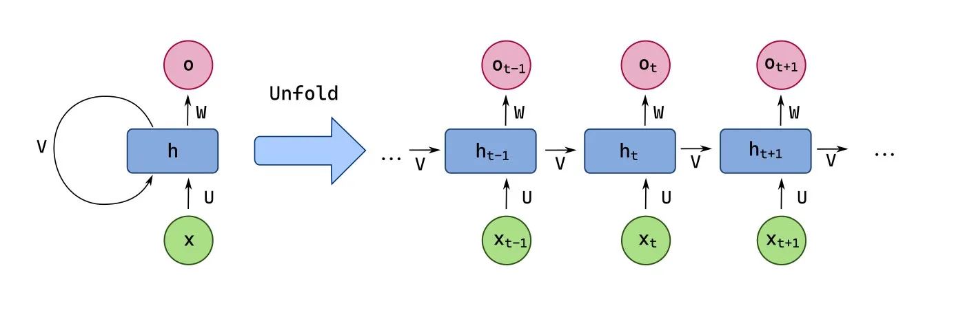
RNNs process sequences step by step, carrying a hidden state forward
Each timestep reuses the same weights to incorporate past context
This simple memory can struggle with long-term dependencies

Notation

Input at time $t$ : $x_t$
Hidden state (memory) at time $t$ : $a_t$
Output at time $t$ : $y_t$
Previous hidden state: $a_{t-1}$

How it works (specific)

RNNs utilise recurrent connections, where the output of a neuron at one time step is fed back as input to the network at the next time step
For a RNN, there are a few things we need to keep track of:
- The current timestep $t$
- The input at the current timestep $x_t$
- The output at the current timestep $y_t$
- The hidden states at the previous timestep $a_{t-1}$ and current timestep $a_t$
Broadly speaking, the RNN can be summarised as a function

f_\theta: (x_t, a_{t-1}) \mapsto (y_t, a_t)

1. Set an initial hidden state $a_0$

The initial hidden state $a_0$ needs to be passed into the first timestep $t=1$
Usually, this is done by setting $a_0 = 0$
Some implementations learn a trainable $a_0$ instead of using zeros
The choice of $a_0$ can affect early outputs for short sequences

2. Calculate the hidden state $a_t$

Using the hidden state of the previous timestep $t-1$ , take an input $x_t$ to calculate $a_t$
The nonlinearity $\phi$ is commonly $\tanh$ or $\mathrm{ReLU}$
Weights are shared across all timesteps, which keeps parameter count fixed

a_t = \phi(W_a a_{t-1} + W_x x_t + b_a)

3. Calculate the output for this timestep $y_t$

Using the hidden state $a_t$ , calculate the output $y_t$
The output can be used at every timestep or only at the final step, depending on the task
A softmax layer is common for classification outputs

y_t = W_y a_t + b_y

4. Pass the current hidden state $a_t$ to the next timestep $t+1$

The current hidden state $a_t$ is passed along to the next timestep as a form of input
Steps 1 to 4 are repeated for all of the sequential data
Backpropagation through time (BPTT) is used to train the parameters
Gradients can explode or vanish as sequence length grows

Practical usage

Short-sequence tasks where long-term memory is not critical (e.g., character-level text, simple sequence classification)
Baseline time-series forecasting or anomaly detection with limited context
Lightweight sequence labelling when model size and speed matter

LSTMs

Core idea (high level)

A standard RNN has one stream of memory that gets overwritten as new inputs arrive
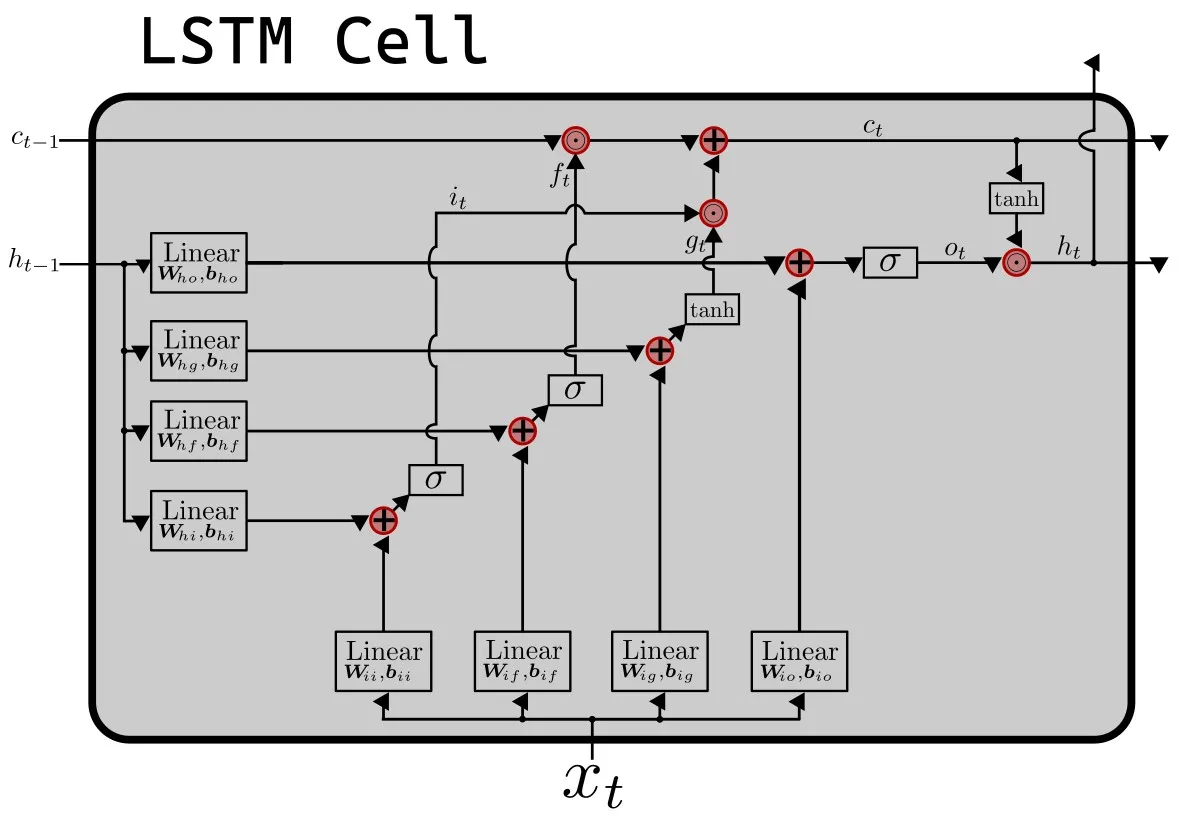
An LSTM adds a separate, protected memory channel and explicit control mechanisms that decide:
- what to keep,
- what to discard,
- what to output at each time step.
This gives superiour control over the memory provided to the model at every timestep, splitting the memory into long-term memory and short-term memory

Notation (gates and memory)

The gates are element-wise values in $[0, 1]$ $[0, 1]$ that control how much information is retained, added, or exposed:
- Forget gate: $f_t$ (how much of $C_{t-1}$ to keep)
- Input gate: $i_t$ (how much new information to write)
- Output gate: $o_t$ (how much of the cell state to expose as output)
Cell state (long-term memory): $C_t$
Hidden state (short-term memory/output): $h_t$
Input at time $t$ : $x_t$

How it works (specific)

1. Set the initial states $h_0$ and $C_0$

Initialise the hidden state and cell state (often zeros).
Some implementations learn $h_0$ and $C_0$ as trainable parameters
These initial states seed the memory for the first timestep

2. Compute the forget gate $f_t$

The forget gate decides how much of $C_{t-1}$ is retained
Values close to 0 drop old information; values close to 1 keep it

f_t = \sigma(W_f [h_{t-1}, x_t] + b_f)

3. Compute the input gate $i_t$ and candidate memory $\tilde{C}_t$

The input gate controls how much new information is written to memory
The candidate memory proposes new content to add

i_t = \sigma(W_i [h_{t-1}, x_t] + b_i)

\tilde{C}_t = \tanh(W_C [h_{t-1}, x_t] + b_C)

4. Update the cell state $C_t$

The cell state blends retained memory with new candidate content
This pathway helps gradients flow across long sequences

C_t = f_t \odot C_{t-1} + i_t \odot \tilde{C}_t

5. Compute the output gate $o_t$

The output gate decides how much of the cell state is exposed
It controls the information sent to the next layer or timestep

o_t = \sigma(W_o [h_{t-1}, x_t] + b_o)

6. Compute the hidden state $h_t$

The hidden state is the short-term, exposed memory
It is what downstream layers typically consume

h_t = o_t \odot \tanh(C_t)

Practical usage

Long-range dependency tasks (e.g., document classification, language modelling, machine translation)
Speech recognition and synthesis, where temporal context matters over many steps
Time-series forecasting with seasonal or delayed effects

GRUs

Core idea (high level)

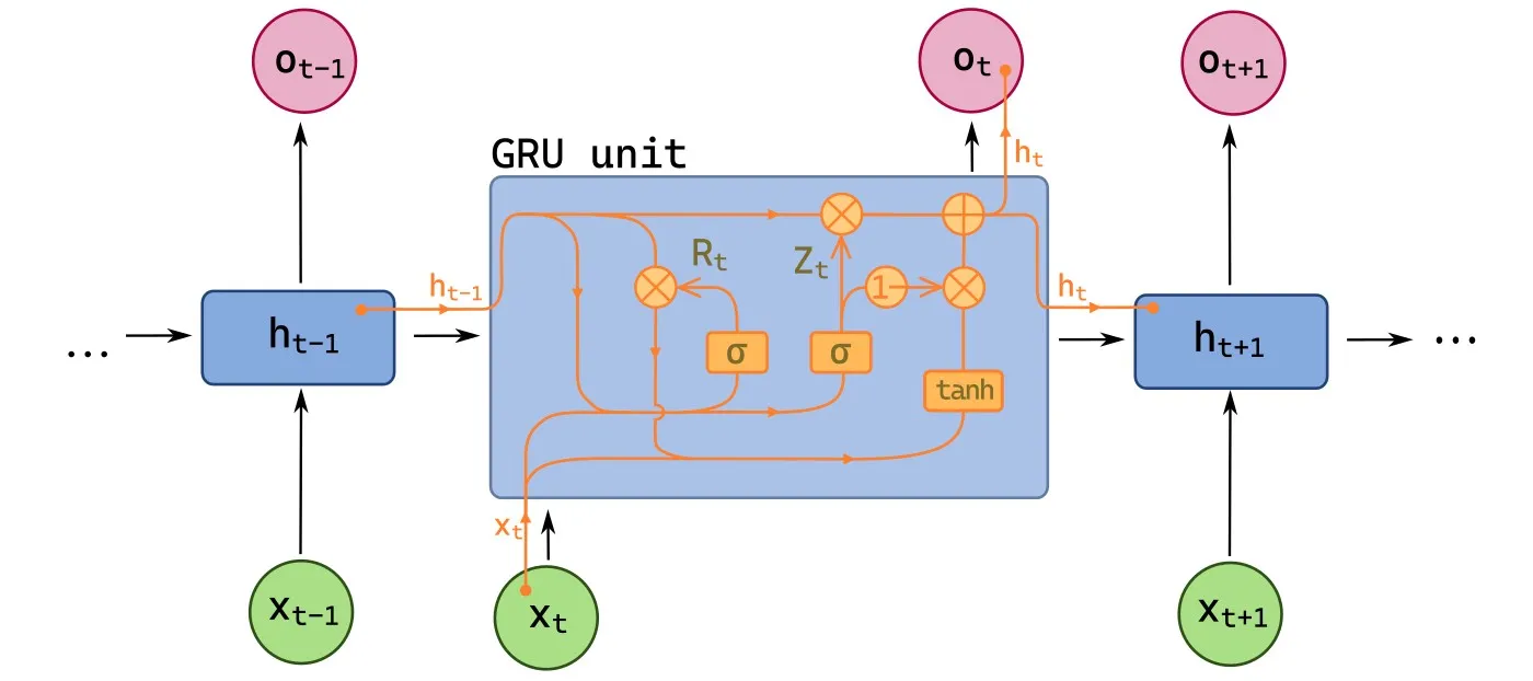
A GRU merges the LSTM’s cell state and hidden state into a single state $h_t$
It uses two gates to control information flow:
- Update gate $z_t$ decides how much past information to keep
- Reset gate $r_t$ decides how much past information to forget when proposing new content
This makes GRUs simpler and often faster than LSTMs while retaining strong performance

Notation (gates and memory)

Update gate: $z_t$ (how much of $h_{t-1}$ to keep)
Reset gate: $r_t$ (how much of $h_{t-1}$ to use in candidate)
Hidden state (memory/output): $h_t$
Candidate hidden state: $\tilde{h}_t$
Input at time $t$ : $x_t$

How it works (specific)

1. Set the initial hidden state $h_0$

Initialise the hidden state (often zeros).
Some implementations learn a trainable $h_0$
This state acts as the initial memory before any inputs

2. Compute the update gate $z_t$

The update gate controls how much of the past is carried forward
Larger $z_t$ values preserve $h_{t-1}$

z_t = \sigma(W_z [h_{t-1}, x_t] + b_z)

3. Compute the reset gate $r_t$

The reset gate controls how much past information influences the candidate
Smaller $r_t$ values push the model to ignore old context

r_t = \sigma(W_r [h_{t-1}, x_t] + b_r)

4. Compute the candidate hidden state $\tilde{h}_t$

The candidate mixes current input with a gated version of past state
It represents the proposed new content for memory

\tilde{h}_t = \tanh(W_h [r_t \odot h_{t-1}, x_t] + b_h)

5. Update the hidden state $h_t$

The final state interpolates between old and candidate states
This interpolation is simpler than the LSTM cell/hidden split

h_t = (1 - z_t) \odot \tilde{h}_t + z_t \odot h_{t-1}

Practical usage

Similar to LSTMs but with fewer parameters, useful for smaller datasets or faster training
Real-time or edge deployments where model size/latency is constrained
Robust baselines for many sequence tasks (e.g., sentiment, tagging, forecasting)

RNNs, LSTMs and GRUs

RNNs, LSTMs, and GRUs

Syllabus Map

Outline

RNNs

Core idea (high level)

Notation

How it works (specific)

1. Set an initial hidden state a0a_0a0​

2. Calculate the hidden state ata_tat​

3. Calculate the output for this timestep yty_tyt​

4. Pass the current hidden state ata_tat​ to the next timestep t+1t+1t+1

Practical usage

LSTMs

Core idea (high level)

Notation (gates and memory)

How it works (specific)

1. Set the initial states h0h_0h0​ and C0C_0C0​

2. Compute the forget gate ftf_tft​

3. Compute the input gate iti_tit​ and candidate memory C~t\tilde{C}_tC~t​

4. Update the cell state CtC_tCt​

5. Compute the output gate oto_tot​

6. Compute the hidden state hth_tht​

Practical usage

GRUs

Core idea (high level)

Notation (gates and memory)

How it works (specific)

1. Set the initial hidden state h0h_0h0​

2. Compute the update gate ztz_tzt​

3. Compute the reset gate rtr_trt​

4. Compute the candidate hidden state h~t\tilde{h}_th~t​

5. Update the hidden state hth_tht​

Practical usage

1. Set an initial hidden state $a_0$

2. Calculate the hidden state $a_t$

3. Calculate the output for this timestep $y_t$

4. Pass the current hidden state $a_t$ to the next timestep $t+1$

1. Set the initial states $h_0$ and $C_0$

2. Compute the forget gate $f_t$

3. Compute the input gate $i_t$ and candidate memory $\tilde{C}_t$

4. Update the cell state $C_t$

5. Compute the output gate $o_t$

6. Compute the hidden state $h_t$

1. Set the initial hidden state $h_0$

2. Compute the update gate $z_t$

3. Compute the reset gate $r_t$

4. Compute the candidate hidden state $\tilde{h}_t$

5. Update the hidden state $h_t$