Syllabus Map

Study map: Syllabus Study Map

Overview

Self-supervised learning builds visual features without manual labels.
The goal is to learn general representations that transfer to classification, detection, and segmentation.

Core Ideas

Pretext Tasks

Predict masked patches (masked image modeling).
Solve contrastive objectives with positive/negative pairs.
Predict rotations, colorization, jigsaw order (classic but less used now).

Representation Learning

Learn embeddings that transfer to downstream tasks.
Evaluate with linear probes, k-NN, or full fine-tuning.

Main Families (Vision)

Contrastive Learning

SimCLR: two augmented views; maximize agreement with InfoNCE loss.
MoCo: momentum encoder + queue of negatives for scalable contrast.
SwAV: online clustering with multi-crop augmentation (no explicit negatives).

Bootstrap / Non-Contrastive

BYOL: online and target networks; stop-gradient avoids collapse.
SimSiam: predictor head + stop-gradient, no negatives.

Masked Image Modeling

MAE: mask large portions of patches, reconstruct pixels with a decoder.
BEiT: predict discrete visual tokens (like a visual vocabulary).

Step-by-Step: Contrastive Learning Objectives

Objective 1: Instance Discrimination (Image-Level)

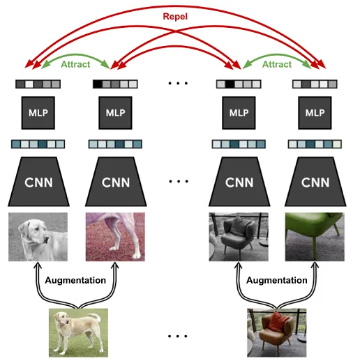
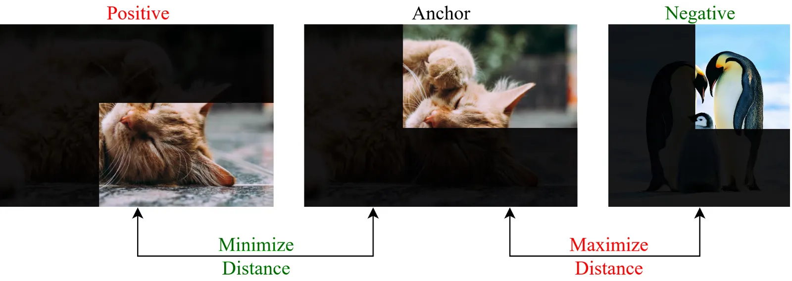
Treat each image instance as its own class using two augmented views.
Pull the positive pair together and push all other images in the batch away.

s(a, b) = \frac{a^T b}{\|a\| \|b\|}

L_i = -\log \left( \frac{\exp(s(z_i, z_i^+) / \tau)} {\sum_{k \ne i} \exp(s(z_i, z_k) / \tau)} \right)

L_{\text{batch}} = \frac{1}{2N} \sum_{i=1}^{2N} L_i

Objective 2: Image Subsampling / Patching (Patch-Level)

Split image features into local patches (or crop local regions) and contrast local positives against negatives.
Positives can be two views of the same patch location/region; negatives are other patches or other images.

L_{\text{patch}}(i, p) = -\log \left( \frac{\exp(s(z_{i,p}^a, z_{i,p}^b) / \tau)} {\sum_{(j,q) \ne (i,p)} \exp(s(z_{i,p}^a, z_{j,q}) / \tau)} \right)

L_{\text{total}} = \lambda_{\text{img}} L_{\text{batch}} + \lambda_{\text{patch}} \frac{1}{P} \sum_{p=1}^{P} L_{\text{patch}}(:, p)

Step-by-Step: Instance Discrimination

Step 1: Sample a Batch

Draw a mini-batch of unlabeled images.
Larger batches provide more in-batch negatives.

Step 2: Create Two Augmented Views

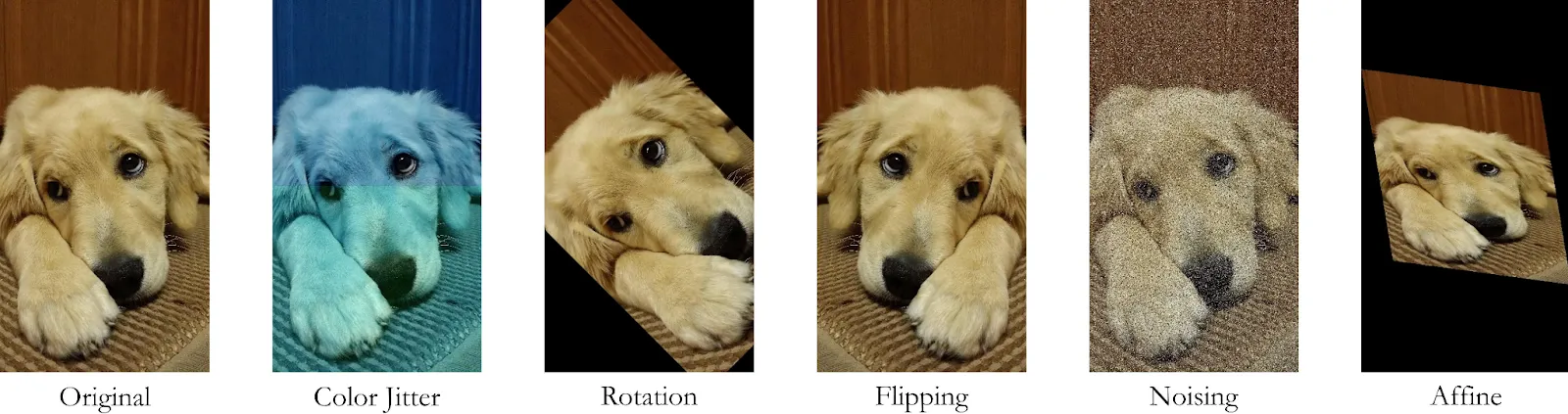
Apply two random augmentation pipelines to each image.
Typical transforms: random crop, color jitter, blur, flip.

Step 3: Encode and Project

Encode each view with a shared encoder $f$ .
Map encoder features through a projection head $g$ to get $z$ .

h_i = f(x_i), \quad z_i = g(h_i)

Step 4: Build Positive/Negative Sets

Positive pair: two views from the same original image.
Negatives: all other views in the current batch (or memory queue in MoCo).

Step 5: Optimize InfoNCE

Compute pair similarities and temperature-scaled softmax.
Backpropagate $L_batch$ to update $f$ and $g$ .

Step 6: Transfer Encoder

Discard $g$ after pretraining.
Use $f$ for linear probing or end-to-end fine-tuning.

Step-by-Step: Image Subsampling / Patching

Step 1: Generate Local Regions or Tokens

Create patches by ViT tokenization or region crops from CNN feature maps.
Produce two views so corresponding patches can be matched.

Step 2: Encode Local Features

Extract patch embeddings from both views.
Optionally add a patch-level projection head.

h_{i,p} = f(x_i, p), \quad z_{i,p} = g_{\text{patch}}(h_{i,p})

Step 3: Define Patch Positives and Negatives

Positive: matched patch/region across two augmented views.
Negatives: unmatched patches in the same image and patches from other images.

Step 4: Compute Patch Contrastive Loss

Apply patch-level InfoNCE for each selected patch.
Average across patches, then combine with image-level loss if used.

L_{\text{total}} = \lambda_{\text{img}} L_{\text{batch}} + \lambda_{\text{patch}} L_{\text{patch\_avg}}

Step 5: Update and Transfer

Optimize encoder and projection heads jointly.
Keep the encoder for downstream dense tasks (segmentation, detection) or classification.

Key Design Choices

Augmentations: random crop, color jitter, blur, solarize, and horizontal flip are critical for contrastive methods.
Backbones: ResNet for early SSL, ViT is now common for MIM.
Projection head: MLP head often improves representation quality.
Losses: InfoNCE for contrastive, cosine regression for BYOL/SimSiam, reconstruction loss for MAE.

Self-Supervised Learning for Vision

Syllabus Map

Overview

Core Ideas

Pretext Tasks

Representation Learning

Main Families (Vision)

Contrastive Learning

Bootstrap / Non-Contrastive

Masked Image Modeling

Step-by-Step: Contrastive Learning Objectives

Objective 1: Instance Discrimination (Image-Level)

Objective 2: Image Subsampling / Patching (Patch-Level)

Step-by-Step: Instance Discrimination

Step 1: Sample a Batch

Step 2: Create Two Augmented Views

Step 3: Encode and Project

Step 4: Build Positive/Negative Sets

Step 5: Optimize InfoNCE

Step 6: Transfer Encoder

Step-by-Step: Image Subsampling / Patching

Step 1: Generate Local Regions or Tokens

Step 2: Encode Local Features

Step 3: Define Patch Positives and Negatives

Step 4: Compute Patch Contrastive Loss

Step 5: Update and Transfer

Key Design Choices

Practical Notes

Data and Compute

Evaluation and Transfer