Syllabus Map

• Study map: Syllabus Study Map

Overview

• The R-CNN family introduced region-based object detection using explicit proposals.
• Each step improved compute reuse and training simplicity.
• The main evolution is: R-CNN → Fast R-CNN → Faster R-CNN.

R-CNN

Core idea

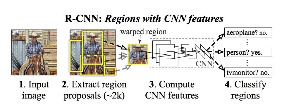
• Generate region proposals, then run a CNN on each proposal.
• Classify each region and refine its box.

Pipeline

• Selective Search proposes ~2k regions per image.
• Warp + CNN: each proposal is warped to a fixed size (e.g., 227x227) and fed through a backbone like AlexNet or VGG.
• SVMs: one-vs-rest linear SVM per class on cached CNN features.
• Box regressor: class-specific linear regressors refine bounding boxes.

How Selective Search Works (Step-by-Step)

Step 1: Initial over-segmentation

• Split the image into many small regions (superpixels) using color/texture boundaries.

Step 2: Compute region similarities

• Score neighboring regions by hand-crafted similarity cues: color histogram, texture, size, and fill.

Step 3: Greedy merging

• Repeatedly merge the most similar neighboring region pair.
• After each merge, recompute similarities with new neighbors.

Step 4: Generate proposals at all hierarchy levels

• Each merged region defines a candidate object region.
• Convert each candidate region to a bounding box proposal.

Step 5: Remove duplicates

• Use simple deduplication and ranking to keep a manageable proposal set (around 2k).

Step 6: Hand off to CNN stage

• R-CNN crops/warps each proposal and runs a separate CNN forward pass per proposal.

Key traits

• Accurate, but extremely slow at inference.
• Multi-stage training: pretrain on ImageNet, fine-tune CNN on detection, then train SVMs + box regressors.
• Heavy disk usage to cache features for all proposals.

Fast R-CNN

Core idea

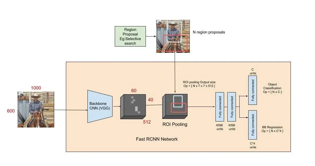
• Run the CNN once per image, then classify regions using pooled features.
• Reuse that shared feature map for all proposals instead of recomputing convolution features per region.

Pipeline

• Backbone CNN produces a shared feature map.
• ROI Pooling converts each ROI into a fixed 7x7 feature map by quantized spatial binning.
• Single head outputs class scores (softmax) + box deltas for each ROI.

Why “CNN Once Per Image” Is Better

• R-CNN bottleneck: if there are ~2k proposals, convolution is run ~2k times per image.
• Fast R-CNN change: run convolution once on the full image, then slice ROI features from the shared map.
• Computation reuse: overlapping proposals share most low/mid-level features, so repeated conv work is removed.
• Memory/I-O improvement: no need to cache per-proposal CNN features to disk.
• Training simplification: classification and box regression are learned jointly from shared features.

Key traits

• Much faster than R-CNN.
• End-to-end training with a multi-task loss (classification + smooth L1 box regression).
• Still depends on external proposals (Selective Search).

Faster R-CNN

Core idea

• Replace external proposal generation with a Region Proposal Network (RPN).

Pipeline

• Backbone CNN shared by RPN and detection head.
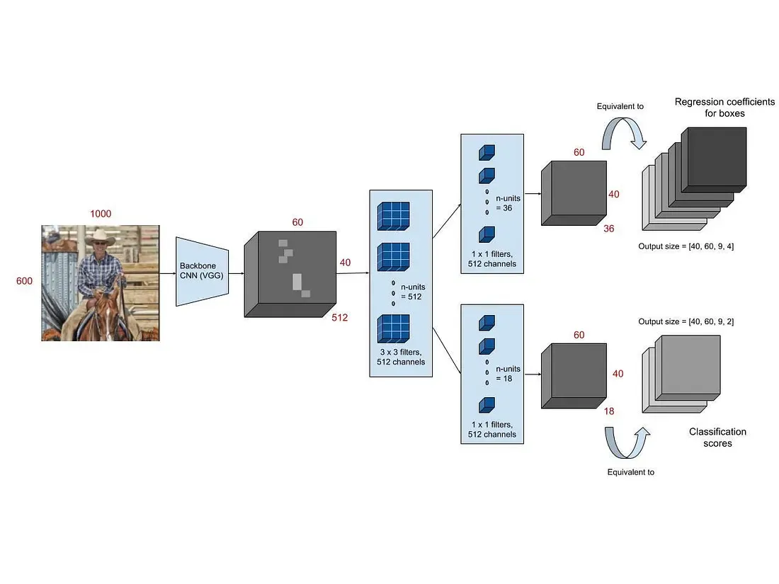
• RPN: a 3x3 conv sliding over the feature map predicts objectness + anchor box offsets.
• Anchors: multiple scales and aspect ratios per location (e.g., 3 scales x 3 ratios).
• ROI Pooling / ROI Align extracts proposal features (ROI Align removes quantization).
• Detection head predicts class + refined box.

How RPN Works (Step-by-Step)

Step 1: Shared feature extraction

• Pass image through the backbone once to get a convolutional feature map.

Step 2: Dense anchor placement

• At each spatial location, place $k$ anchor boxes with predefined scales and aspect ratios.

Step 3: Sliding prediction heads

• A small RPN head predicts for each anchor:
  • Objectness score (foreground vs background),
  • Box regression offsets $(\Delta x, \Delta y, \Delta w, \Delta h)$.

Step 4: Anchor labeling (training)

• Match anchors to ground-truth boxes by IoU thresholds to mark positive/negative anchors.
• Train with combined objectness + box regression loss.

Step 5: Proposal decoding

• Convert anchor + predicted offsets into proposal boxes in image coordinates.
• Clip boxes to image boundaries and remove tiny/invalid boxes.

Step 6: Proposal filtering

• Rank proposals by objectness, apply NMS, keep top proposals (for example top 300 at inference).

Step 7: Hand-off to detector

• Send filtered proposals to ROI Pooling/ROI Align and then to the final classification/regression head.

Key traits

• Fully end-to-end and much faster than Fast R-CNN.
• Strong accuracy-speed tradeoff for general detection.
• Typical inference keeps ~300 proposals after NMS (config dependent).

Mask R-CNN

Core idea

• Extend Faster R-CNN with a parallel segmentation mask prediction branch.

Pipeline

• Backbone + FPN often used to improve multi-scale features.
• RPN generates proposals as in Faster R-CNN.
• ROI Align replaces ROI Pooling to avoid misalignment from quantization.
• Two heads: class + box regression, and a small FCN mask head that predicts a K x m x m mask per class.

Key traits

• Adds instance segmentation with minimal overhead.
• Mask loss is per-pixel sigmoid (not softmax across classes).
• Requires precise ROI alignment for good mask quality.

How They Differ

• R-CNN: per-region CNN, SVMs, slow.
• Fast R-CNN: shared CNN, ROI Pooling, still external proposals.
• Faster R-CNN: shared CNN + built-in RPN proposals.
• Mask R-CNN: Faster R-CNN + mask head with ROI Align.

Training Objectives (High Level)

• Classification loss: object class per ROI.
• Box regression loss: refine bounding box coordinates.
• RPN loss (Faster R-CNN only): objectness + anchor box offsets.

When To Use

• R-CNN: historical baseline, rarely used now.
• Fast R-CNN: useful for understanding the progression.
• Faster R-CNN: strong default for accurate detection.

Practical Notes

Use stable optimization defaults first

• Fast R-CNN and Faster R-CNN are commonly trained with SGD, momentum around 0.9, and weight decay around $5\times10^{-4}$ in classic settings.
• Start with proven optimizer settings before tuning advanced schedules.
• Monitor classification and box regression losses separately to diagnose imbalance.

Understand training strategy differences

• Early Faster R-CNN recipes often used alternating stages: train RPN, train detector, then joint fine-tuning.
• Modern implementations typically support more direct end-to-end training, but alternating training remains useful context.
• Keep proposal quality and detector quality aligned during training to avoid bottlenecks.

Prioritize compute-efficient architectures in practice

• R-CNN-style per-proposal CNN inference can require around 2k forward passes per image, which is computationally expensive.
• Fast R-CNN improves speed by sharing one feature map across proposals.
• Faster R-CNN further improves the pipeline by learning proposals with the RPN instead of external selective search.