Syllabus Map

• Study map: Syllabus Study Map

Overview

• Generative models synthesise realistic images.
• Two major families are GANs and diffusion models.
• GANs are usually faster at sampling; diffusion models are usually more stable and higher quality.

GAN (Generative Adversial Network)

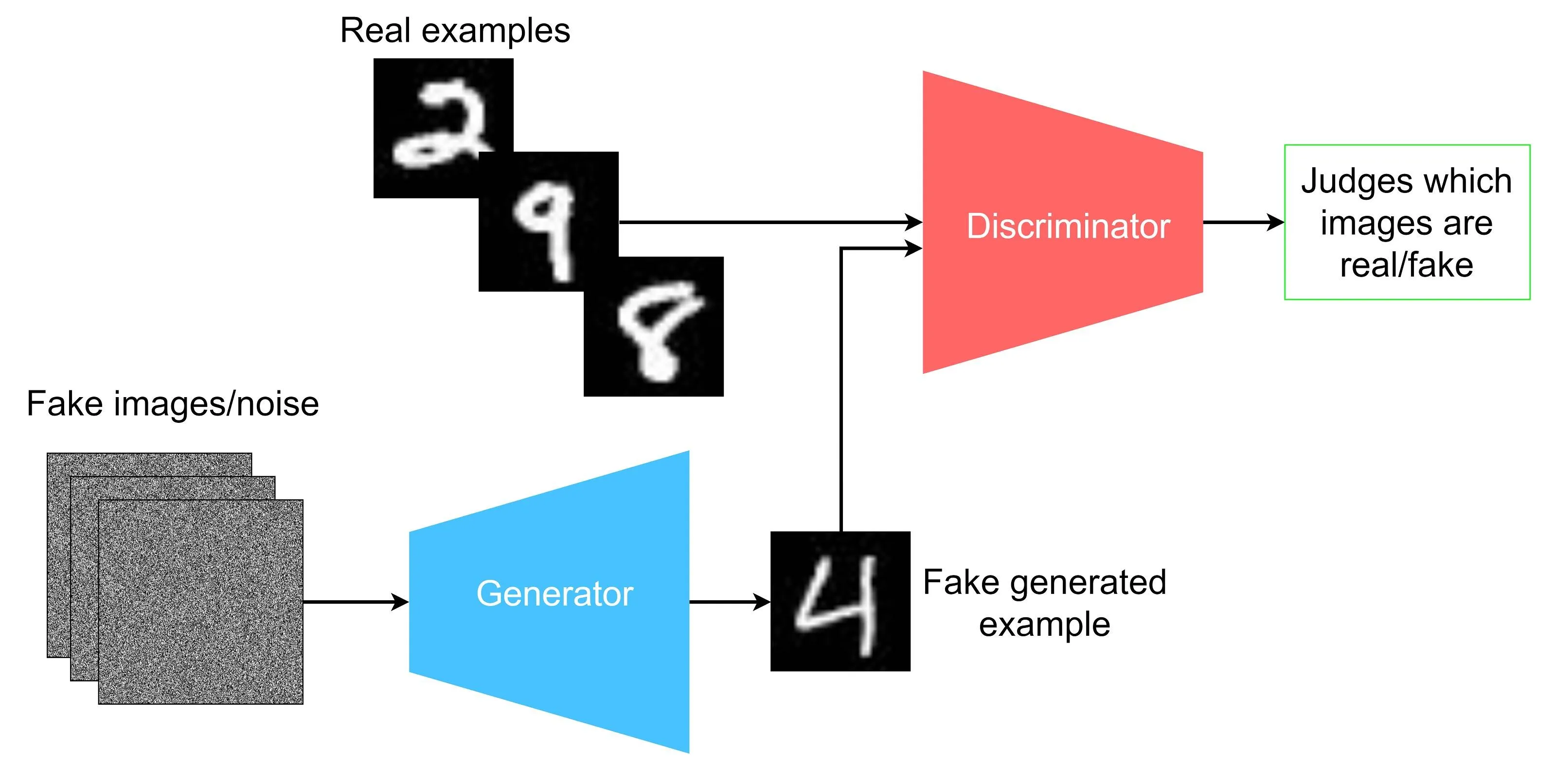
Core Idea

• Generator $G$ maps latent noise $z$ to an image $\hat{x}=G(z)$.
• Discriminator $D$ predicts whether an image is real ($x$) or generated ($G(z)$).
• Training is adversarial:

• $p_{\text{data}}$ is the real image distribution.
• $p(z)$ is latent prior (typically Gaussian).

Step-by-Step GAN Training

Step 1: Sample data and latent vectors

• Draw real images $x$ from the dataset.
• Draw noise vectors $z\sim \mathcal{N}(0,I)$.

Step 2: Update discriminator

• Train $D$ to assign high score to real images and low score to generated images.
• This improves real/fake separation.

Step 3: Update generator

• Train $G$ to produce images that fool $D$.
• Generator gradients flow through discriminator feedback.

Step 4: Alternate updates

• Repeat discriminator and generator updates.
• Keep training balanced to avoid one network overpowering the other.

Important GAN Variants

• DCGAN: convolutional baseline for stable image generation.
• WGAN / WGAN-GP: Wasserstein objective + gradient penalty for improved stability.
• StyleGAN2/3: style-based generator with strong photorealism and controllability.

Practical Notes

Training stability is the main challenge

• GAN optimization can oscillate or diverge if updates are not balanced.

Balance generator and discriminator updates

• Keep $G$ and $D$ learning rates and update frequencies well matched.

Watch for mode collapse

• Generated samples may lose diversity even when quality appears high.
• Mode collapse means the generator finds a small set of outputs that reliably fool the discriminator and keeps repeating that pattern.
• If one “good enough” dog image keeps fooling $D$, $G$ may stop learning other dogs and keep producing near-duplicates.

Track quality with standard metrics

• FID and IS are common diagnostics alongside qualitative inspection.

Diffusion Models

Core Idea

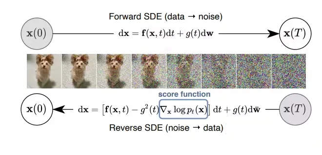
Denoising Process

• Learn to denoise from random noise to a data sample.
• Forward process gradually adds Gaussian noise to images.
• Reverse process learns to remove noise step-by-step.

Markov Formulation

• The diffusion process is a Markov chain: each state depends only on the previous state, i.e., $q(x_t \mid x_{t-1})$.
• Here, $x_{t-1}$ is the sample at the previous step, $x_t$ is the noisier sample at step $t$, and $\beta_t$ is the step-$t$ noise variance.

Model Components

• In most modern diffusion models, the denoiser is a U-Net that predicts noise at each timestep.
• In latent diffusion (for example Stable Diffusion), a VAE encodes images into latent space before diffusion and decodes latents back to pixels after denoising.

Text Conditioning

• Text-conditioned models commonly use a CLIP text encoder to convert the prompt into embeddings used to condition the U-Net (typically via cross-attention).

Step-by-Step Diffusion Training

Step 1: Sample image and timestep

• Draw clean image $x_0$ (original data sample) and random timestep $t \in \{1,\dots,T\}$.

Step 2: Add noise

• Sample $\epsilon \sim \mathcal{N}(0,I)$ and form noisy sample:

• $\epsilon$ is sampled Gaussian noise, and $\bar{\alpha}_t = \prod_{s=1}^{t}(1-\beta_s)$ is the cumulative signal-retention factor up to step $t$.

Step 3: Predict noise

• Train denoiser $\epsilon_\theta(x_t,t,c)$ to estimate the injected noise.
• $\epsilon_\theta(\cdot)$ is the model’s predicted noise, and $c$ is optional conditioning input (for example text prompt).

Step 4: Optimize denoising loss

Step 5: Sample images

• Start from $x_T\sim \mathcal{N}(0,I)$, where $x_T$ is the near-pure noise state at the final diffusion step.
• Iteratively denoise from timestep $T$ down to $0$.

Guidance and Samplers

Classifier Guidance (Older Approach)

• Before CFG, diffusion models used an external classifier $p_\phi(c\mid x_t)$ to guide sampling toward class $c$.
• The reverse update adds a classifier gradient term that pushes samples toward higher class probability.
• This improves condition fidelity but needs a separate noisy-image classifier and can reduce sample diversity.

Classifier-free guidance (CFG)

• During training, randomly drop the condition $c$ some fraction of the time so the same model learns both conditioned and unconditioned predictions.

• At inference, run the model twice (conditioned and unconditioned) and combine them with guidance scale $w$.
• $\varnothing$ denotes unconditioned input, and $w$ is guidance scale; larger values strengthen condition fidelity but can reduce diversity.
• Common samplers: DDPM, DDIM, and DPM-Solver variants.

DDIM (Denoising Diffusion Implicit Models)

• DDIM uses a non-Markovian reverse process that can sample with fewer steps than DDPM.
• It can be deterministic ($\eta=0$), which makes generation faster and more consistent for the same seed.
• A common DDIM update is:

• Setting $\sigma_t=0$ (equivalently $\eta=0$) gives deterministic sampling; larger $\eta$ adds stochasticity and diversity.

Inpainting

• Inpainting generates missing or edited regions while preserving unmasked context.
• Provide the original image and a binary mask; the model denoises mainly inside masked areas and keeps known pixels fixed.
• This is useful for object removal, region editing, and prompt-based local modifications.

Practical Notes

Delivers strong image quality

• Diffusion models are often strong on realism and diversity.

Inference is usually slower than GANs

• Multiple denoising steps increase latency compared with one-pass generators.

Latent diffusion improves efficiency

• Denoising in compressed latent space reduces memory and compute cost.

Tune sampler controls carefully

• Noise schedule, denoising steps, guidance scale, and sampler strongly affect output behavior.

GANs vs Diffusion (Quick Comparison)

• Training stability: diffusion usually easier to optimize.
• Sampling speed: GANs are usually faster (single pass).
• Quality/diversity: modern diffusion is usually stronger.
• Conditioning: diffusion integrates text/image guidance naturally.