Syllabus Map

• Study map: Syllabus Study Map

Overview

• Convolutions extract local spatial patterns.
• Stacking layers builds hierarchical visual features.
• Residual connections help train deeper CNNs by improving gradient flow.

Convolution Basics

Core Idea

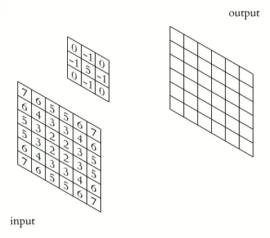
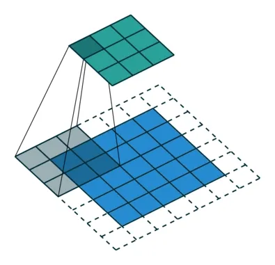
• Apply a learnable filter across the image.
• Capture edges, textures, and shapes.
• Weight sharing reduces parameters and improves translation robustness.

Key Concepts

Kernels

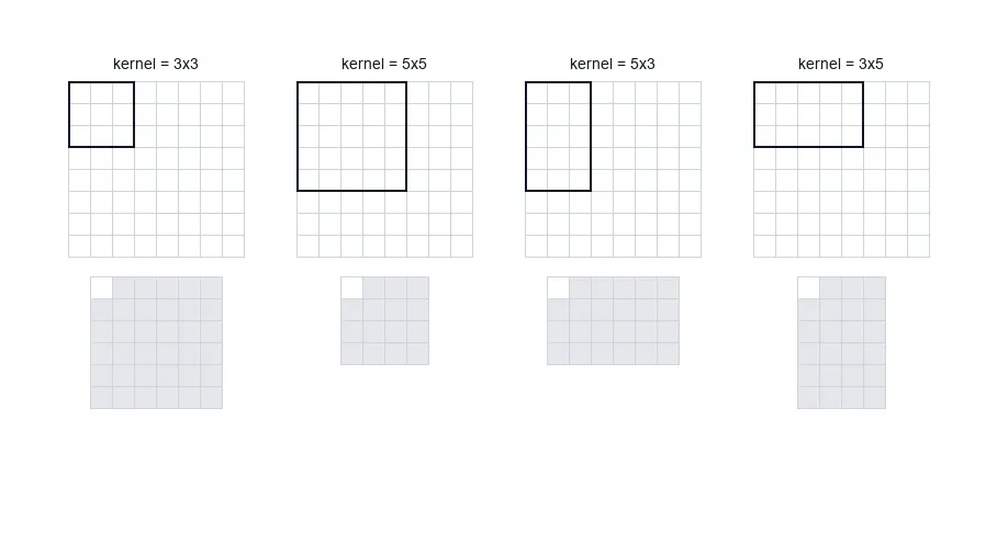
• A kernel is a small window of learnable weights.
• It slides across the input to detect local patterns.
• Kernel size controls how much context the filter sees.

Stride

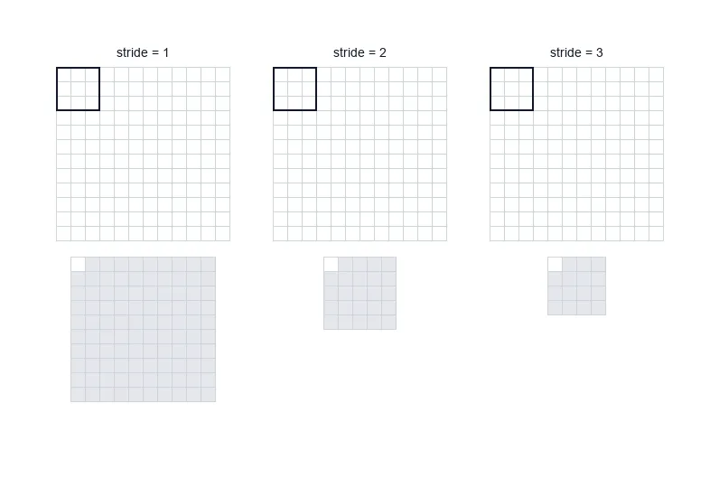
• Controls how far the kernel moves each step.
• Larger stride reduces spatial resolution.

Padding

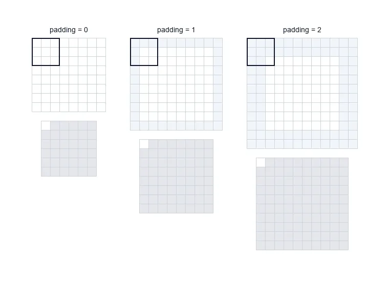
• Adds border pixels to preserve spatial size.
• Helps retain edge information.

Output size

• Depends on input size, kernel size, stride, and padding.

• Use the formula below to compute $H_{out}$ and $W_{out}$.

• For input size $H \times W$:

• $H, W$: input height and width.
• $K$: kernel size (assume square kernel for simplicity).
• $P$: padding size on each side.
• $S$: stride.
• $H_{out}, W_{out}$: output height and width.

Channels and feature maps

• Input channels match the input (e.g., 3 for RGB).
• Output channels are different learned filters.
• Each output channel is a feature map highlighting a pattern.

Convolution operation

• For input $x$ and kernel $w$:

• $y_{i,j}$: output value at spatial location $(i,j)$.
• $w_{u,v}$: kernel weight at offset $(u,v)$.
• $x_{i+u, j+v}$: input value under the kernel at position $(i,j)$.
• The sum is over the kernel window offsets $u,v$.

CNN Overview (General Structure)

Typical pipeline

• Input image (H × W × C).
• Stem: conv + norm + activation to get early edges/textures.
• Stages: repeated conv blocks with occasional downsampling (stride or pooling).
• Head: global pooling + linear classifier (or task-specific heads).

Spatial hierarchy

• Early layers: edges and corners.
• Mid layers: textures and parts.
• Deep layers: objects and semantics.

CNN vs Fully Connected (FC)

Why CNNs dominate for images

• Local connectivity: filters see small neighborhoods first.
• Weight sharing: same filter across the image cuts parameters.
• Translation tolerance: same pattern can be detected anywhere.
• Parameter efficiency: FC layers explode in size for high-res inputs.

When FC makes sense

• Small, fixed-size tabular inputs.
• As a final classifier head after convolutional features.

Residual Connections

Core idea

• Residual blocks add the input back to the output:

• This helps gradients flow and enables very deep networks.

Why residual learning helps

• Degradation problem: very deep plain CNNs can have higher training Error than shallower ones.
• Learning a residual $F(x)$ is often easier than learning a full mapping $H(x)$ directly.
• If the optimal mapping is close to identity, then $H(x) \approx x$ and the residual $F(x) = H(x) - x \approx 0$, which is easier to optimise.

Identity vs projection shortcuts

• Identity shortcut: $y = F(x) + x$ (same shape).
• Projection shortcut: use $1 \times 1$ conv to match channels/stride:
  • $y = F(x) + W_s x$.
  • Used when changing resolution or channel count.

Gradient flow

• Skip connections create short paths for gradients.
• They reduce vanishing gradients but do not eliminate them completely.
• Optimisation becomes easier even if generalisation stays similar.

PyTorch Implementation

Core building blocks

import torch
import torch.nn as nn

conv = nn.Conv2d(in_channels=3, out_channels=32, kernel_size=3, stride=1, padding=1)
bn = nn.BatchNorm2d(32)
relu = nn.ReLU()
pool = nn.MaxPool2d(kernel_size=2, stride=2)

A simple CNN block

class ConvBlock(nn.Module):
    def __init__(self, in_ch, out_ch):
        super().__init__()
        self.net = nn.Sequential(
            nn.Conv2d(in_ch, out_ch, 3, padding=1),
            nn.BatchNorm2d(out_ch),
            nn.ReLU(),
            nn.MaxPool2d(2)
        )

    def forward(self, x):
        return self.net(x)

Residual block (basic)

class ResidualBlock(nn.Module):
    def __init__(self, channels):
        super().__init__()
        self.conv1 = nn.Conv2d(channels, channels, 3, padding=1)
        self.bn1 = nn.BatchNorm2d(channels)
        self.conv2 = nn.Conv2d(channels, channels, 3, padding=1)
        self.bn2 = nn.BatchNorm2d(channels)
        self.relu = nn.ReLU()

    def forward(self, x):
        out = self.relu(self.bn1(self.conv1(x)))
        out = self.bn2(self.conv2(out))
        return self.relu(out + x)

Dataset processing (PyTorch)

Basic image dataset

from torchvision import datasets, transforms

transform = transforms.Compose([
    transforms.Resize((224, 224)),
    transforms.ToTensor(),
    transforms.Normalize(mean=[0.485, 0.456, 0.406],
                         std=[0.229, 0.224, 0.225])
])

train_ds = datasets.ImageFolder("data/train", transform=transform)
val_ds = datasets.ImageFolder("data/val", transform=transform)

DataLoader

from torch.utils.data import DataLoader

train_loader = DataLoader(train_ds, batch_size=32, shuffle=True, num_workers=2)
val_loader = DataLoader(val_ds, batch_size=32, shuffle=False, num_workers=2)