Syllabus Map

• Study map: Syllabus Study Map

Overview

• CNNs are used for image-level prediction, region-level localization, and pixel-level labeling.
• The output granularity determines the task:
• Image classification: one label per image.
• Object detection: boxes + labels per object.
• Image segmentation: label per pixel.

Image Classification

Core Idea

• Input: full image tensor $H \times W \times C$.
• Output: class probability vector of size $K$.
• Train with cross-entropy on labeled images.
• Evaluate with top-1/top-5 accuracy and confusion matrix.

Object Detection

Core Idea

• Input: image with variable number of objects.
• Output: $(x, y, w, h, \text{class}, \text{confidence})$ per detected object.
• Train with multi-part loss: classification + box regression (+ objectness).
• Evaluate with mAP at different IoU thresholds (for example, mAP@0.5 and mAP@[0.5:0.95]).

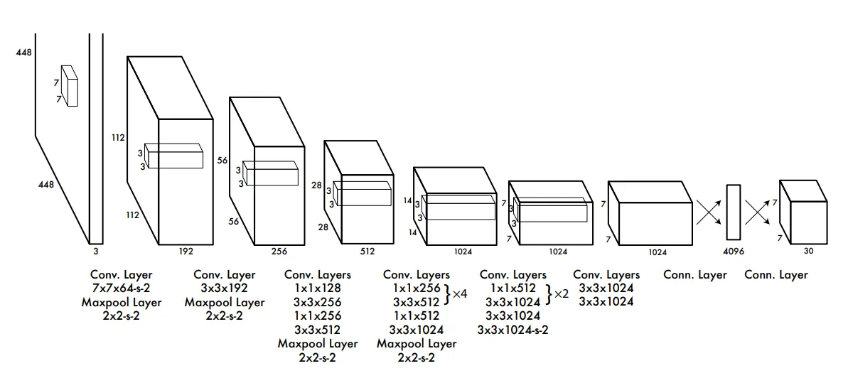
You-Only-Look-Once (YOLO)

Step 1: Prepare Labels

• Convert annotations to normalized box format $(c_x, c_y, w, h, \text{class\_id})$.
• Ensure class IDs are contiguous and images/labels are paired correctly.

Step 2: Train Grid-Based Predictions

• Split image into feature grid cells.
• Predict objectness, class scores, and box offsets per anchor/location.

Step 3: Optimize Detection Loss

• Compute objectness loss for object/background.
• Compute class loss for positive samples.
• Compute box loss (IoU-based or L1-style, depending on YOLO version).
• A common multi-part objective is:

• Where: box/objectness/class losses are weighted by $\lambda_{\text{box}}, \lambda_{\text{obj}}, \lambda_{\text{cls}}$.

• Where: $\text{Pos}$ are matched positive anchors; higher IoU gives lower box loss.

• Binary cross-entropy over object/background labels ($y_i$) and objectness predictions ($p_i$).

• Cross-entropy on class predictions for positive anchors only.

Step 4: Run Post-Processing

• Filter low-confidence predictions.
• Compute overlap with Intersection over Union (IoU):

• IoU ranges from 0 (no overlap) to 1 (perfect overlap).
• Apply Non-Maximum Suppression (NMS) to remove duplicate detections:
  • Sort boxes by confidence score.
  • Keep the highest-score box and suppress lower-score boxes that overlap it too much.
  • Repeat until no candidate boxes remain.

• Keep higher-score box $b_i$ and suppress overlapping lower-score boxes above threshold $\tau_{\text{nms}}$.

Step 5: Evaluate and Deploy

• Measure mAP and latency.
• Tune confidence/NMS thresholds for task-specific precision-recall tradeoff.

Single Shot MultiBox Detector (SSD)

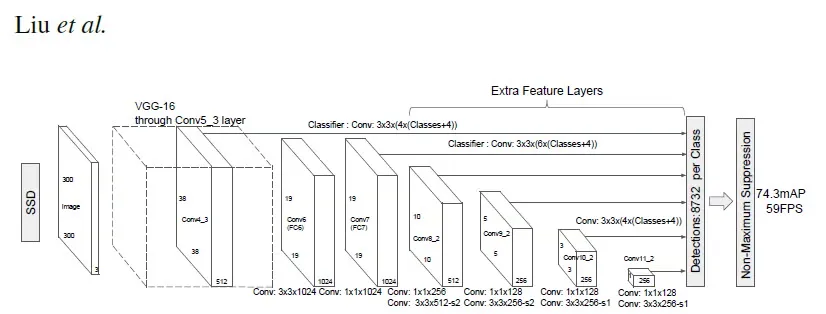
Step 1: Build Multi-Scale Feature Maps

• Extract backbone features at several spatial resolutions.
• Attach detection heads to each scale for small-to-large objects.

Step 2: Match Ground Truth to Default Boxes

• Predefine default boxes (anchors) with multiple scales/aspect ratios.
• Match anchors to ground-truth boxes using IoU rules.

Step 3: Train Classification and Localization

• Predict class logits for each anchor.
• Predict box offsets relative to matched default boxes.
• Typical SSD objective:

• Where: $N$ is number of matched positives, and $\alpha$ balances localization vs classification.

• SmoothL1 regression over box center/size offsets for positive anchors.

Step 4: Apply Hard Negative Mining

• Keep informative negative anchors with highest classification loss.
• Balance positive and negative samples during training.
• Standard ratio target is:

• At most 3 negatives per positive anchor during hard negative mining.

Step 5: Decode and Filter Predictions

• Convert offsets back to absolute boxes.
• Apply confidence thresholding and NMS before final outputs.

Detection Transformers (DETR)

Step 1: Encode Image Features

• Run image through a CNN backbone to get feature maps.
• Flatten features and add positional encodings.

Step 2: Decode with Object Queries

• Feed learned object queries into a transformer decoder.
• Each query predicts one potential object slot.

Step 3: Hungarian Matching

• Match predictions to ground-truth objects one-to-one.
• Use matching cost from class and box terms.
• Matching is solved by:

• Matching cost combines class confidence, L1 box distance, and GIoU overlap.

Step 4: Optimize Set Prediction Loss

• Train class predictions including a “no-object” class.
• Train box regression with L1 + generalized IoU loss.
• DETR set loss:

• Set prediction loss = class loss (with no-object) + weighted L1/GIoU box losses.

Step 5: Inference without NMS

• Keep high-confidence query outputs directly.
• One-to-one matching behavior reduces duplicate detections.

Image Segmentation

Core Idea

• Input: image and dense pixel mask labels.
• Output: mask $H \times W$ (semantic) or per-instance masks (instance segmentation).
• Train with pixel-wise losses (cross-entropy, Dice, or combined loss).
• Evaluate with IoU (Jaccard), Dice score, and pixel accuracy.

Semantic vs Instance Segmentation

Semantic Segmentation

• Assigns a class label to every pixel.
• Pixels from different objects of the same class share one label region.
• Example: all person pixels are labeled “person” without separating person A vs person B.

Instance Segmentation

• Assigns both class and instance identity to pixels.
• Different objects of the same class get separate masks.
• Example: each person in the scene gets its own mask (person 1, person 2, …).

U-Net

Step 1: Encode Context

• Downsample with convolution blocks to capture global context.
• Store intermediate feature maps for skip connections.

Step 2: Decode Spatial Detail

• Upsample progressively back to image resolution.
• Concatenate decoder features with matching encoder skip features.

Step 3: Predict Pixel Masks

• Use final convolution layer to output per-pixel class logits.
• Convert logits to masks with softmax/sigmoid.

Step 4: Train with Dense Losses

• Use cross-entropy for multi-class segmentation.
• Add Dice loss when classes are imbalanced or objects are thin/small.
• Common combined objective:

• Combined segmentation loss: pixel-wise CE + weighted Dice overlap loss.

• $p_i$ and $y_i$ are predicted and ground-truth mask values; $\epsilon$ stabilizes division.

Step 5: Post-Process Masks

• Apply thresholding for binary masks.
• Use connected components or morphology to clean noisy regions.