Syllabus Map
- Study map: Syllabus Study Map
Overview
- t-SNE and UMAP are nonlinear techniques for visualising high-dimensional data.
- Both focus on preserving local structure in low-dimensional projections.
t-SNE (T-distributed Stochastic Neighbour Embedding)
Core Idea
- t-SNE builds a 2D/3D map that keeps nearby points in the original space nearby in the embedding.
- It prioritises local neighborhoods over global geometry.
How It Works (Step-by-Step)
Step 1: Compute High-Dimensional Similarities
- For each point , convert distances to conditional probabilities:
- The bandwidth is chosen so that the perplexity of matches a target value.
- Perplexity is a parameter that sets the effective number of neighbours each point should have in t‑SNE.
- This represents how likely point would “choose” point as a neighbour if neighbours were sampled from a Gaussian centred at .
Step 2: Symmetrise the Probabilities
- Convert conditionals to joint probabilities:
- This yields a symmetric similarity matrix that sums to 1.
- represents mutual similarity, which is how strongly and are neighbours of each other in the original space.
Step 3: Define Low-Dimensional Similarities
- Place points in 2D/3D and define:
- The Student‑t distribution (heavy‑tailed) prevents crowding in low dimensions.
- is a score for how close two points look in the 2D/3D map for all data points, turned into a probability.
Step 4: Optimise the Embedding
- Minimise KL divergence between the two distributions:
- KL divergence (Kullback–Leibler divergence) measures how different one probability distribution is from another.
- It is neither symmetric nor a true distance.
- It tells you how much “information” is lost when you approximate one distribution with another.
- Use gradient descent (often with momentum) to update .
Practical Notes
Hyperparameter Sensitivity
- Sensitive to perplexity and learning rate.
Primary Use Case
- Typically used for visualisation, not downstream modelling.
Limitations
- In t-SNE plots, the distance between separate clusters is usually not meaningful.
- You can interpret which points are local neighbours, but not absolute spacing or relative gaps between far-apart groups.
- t-SNE can show splintering, where one true cluster is broken into multiple small islands due to:
- Hyperparameter choices
- Noise
- Optimisation randomness
- Because of splintering, visual clusters in 2D should be validated against the original high-dimensional structure before making conclusions.
UMAP (Uniform Manifold Approximation and Projection)
Core Idea
- UMAP builds a high‑dimensional neighbour graph, then builds a low‑dimensional graph from the embedding.
- It trains the embedding so the low‑dimensional graph matches the high‑dimensional graph.
- This balances local structure with some global geometry.
How It Works (Step-by-Step)
Step 1: Build the k-NN Graph
- For each point , find its nearest neighbours under the chosen metric.
- This defines a weighted graph over the data.
Step 2: Compute Fuzzy Membership Strengths
- Convert distances into edge probabilities:
- ensures each point has a zero-distance neighbour; controls local connectivity.
- “Fuzzy” means neighbours are not binary; instead each edge has a membership strength between 0 and 1.
Step 3: Construct the Low-Dimensional Fuzzy Graph
- Initialise low‑dimensional points .
- Common initialisation choices:
- Spectral (common default): uses a spectral layout from the graph structure.
- Random: starts points from random positions.
- PCA: starts from a PCA projection.
- Custom init: uses user-provided initial coordinates.
- For low-dimensional points , define:
- Parameters are chosen based on
min_distand the desired embedding smoothness.
Step 4: Optimise by Matching Graphs
- Minimise cross‑entropy between and :
- Use stochastic gradient descent with negative sampling for efficiency.
Intuition
- Think of UMAP as turning data into a network of nearby points, then finding a 2D/3D layout that keeps neighbours close.
- Points that are strongly connected stay close; weakly connected points can drift apart.
Key Hyperparameters
n_neighbors: controls local vs. global structure (smaller = more local).min_dist: controls how tightly points pack in the embedding (smaller = tighter clusters).metric: defines distance in the original space (e.g.,euclidean,cosine).
Practical Notes
Runtime on Large Datasets
- Faster than t-SNE for larger datasets.
Global Structure Preservation
- Often preserves more global structure than t-SNE.
Supervised and Semi-Supervised UMAP
- UMAP can be run in a supervised or semi-supervised mode, where target labels are used to influence the neighbour graph and pull same-label points closer in the embedding.
- This often improves class separation for visualisation, but can hide true unsupervised structure if labels are noisy or incomplete.
Fit/Transform Workflow
- Fit on training data only; transform validation/test consistently.
Axis Interpretability
- Embeddings are nonlinear and not directly interpretable as feature axes.
PCA vs t-SNE vs UMAP
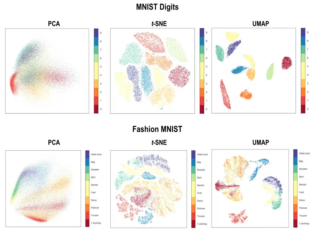
Quick Comparison
| Method | Type | What It Preserves Best | Speed | Typical Use |
|---|---|---|---|---|
| PCA | Linear projection | Global variance structure | Fastest | Compression, preprocessing, baseline visualisation |
| t-SNE | Nonlinear embedding | Local neighbourhoods | Slowest | Visual cluster inspection |
| UMAP | Nonlinear manifold/graph embedding | Local structure + some global geometry | Medium | Visualisation and sometimes downstream features |
Key Takeaways
- PCA is best when you want a simple, stable linear reduction.
- t-SNE is best for local cluster visualisation, but inter-cluster distances are not reliable.
- UMAP often gives a better speed/structure tradeoff and supports supervised guidance.