Syllabus Map

Study map: Syllabus Study Map

Overview

Support Vector Machines (SVMs) are effective out-of-the-box classifiers.
SVM is also a generalisation of the maximal margin classifier.
Assuming we have a dataset with two classes, we want to find the optimal hyperplane which can separate the two classes.
The margin refers to the minimum distance between two data points of two different classes perpendicular to the direction of the hyperplane.

What is a Hyperplane?

For a hyperplane in $p$ dimensions, it is defined as a flat affine subspace with $p - 1$ dimensions.
In other words, a hyperplane can be thought of as a decision boundary.

Defining the separating hyperplane

Assume we have a dataset in a two-dimensional space which can be linearly separated, the hyperplane dividing the data points according to their classes is a line.
The hyperplane $H_0$ can be defined as the set of points $x$ which satisfy the equation:

w_1 x_1 + w_2 x_2 + \cdots + w_p x_p + b = 0

If we select two hyperplanes $H_1$ and $H_2$ with the same distance from $H_0$ , and ensuring that each data point lies on the correct side with no data in between, they can be defined as:

(H_1)\space w_1 x_{i1} + w_2 x_{i2} + \cdots + w_p x_{ip} + b \ge 1 \quad \text{if } y_i = 1

(H_2)\space w_1 x_{i1} + w_2 x_{i2} + \cdots + w_p x_{ip} + b \le -1 \quad \text{if } y_i = -1

Where:
- $x_i = (x_{i1}, x_{i2}, \dots, x_{ip}) \in \mathbb{R}^p$
- $y_i \in \{-1, 1\}$

Finding the optimal separating hyperplane

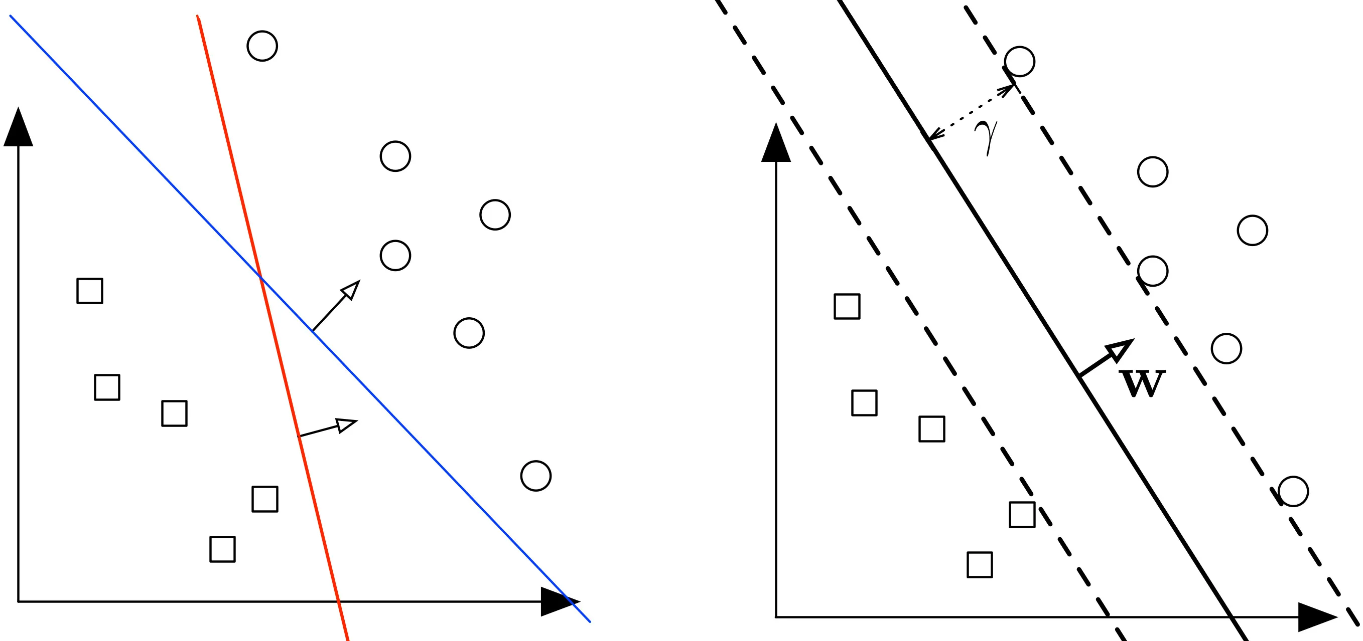
Since our dataset can be perfectly separated using a hyperplane and any hyperplane can be shifted and rotated, there are an infinite number of possible solutions.
The optimal separating hyperplane is the solution that is farthest away from the closest data point, or maximises the margin.

Defining the margin

In order to maximise the distance between the two hyperplanes, we need to find a way to calculate the margin.
The margin can also be interpreted as a direction perpendicular to the hyperplane with a magnitude equal to the margin.

1. Distance from a point to a hyperplane

For any point $x = (x_1, x_2, \dots, x_p)$ , the distance to the hyperplane
$w_1 x_1 + w_2 x_2 + \cdots + w_p x_p + b = 0$ is:

d = \frac{| w_1 x_1 + w_2 x_2 + \cdots + w_p x_p + b |} {\sqrt{w_1^2 + w_2^2 + \cdots + w_p^2}}

2. Distance between the two margin hyperplanes

The margin hyperplanes are:

\text{(H1) } w_1 x_1 + w_2 x_2 + \cdots + w_p x_p + b = 1

\text{(H2) } w_1 x_1 + w_2 x_2 + \cdots + w_p x_p + b = -1

Thus, the distance between two parallel hyperplanes is:

\gamma \space \text{(margin)} = \frac{2}{\sqrt{w_1^2 + w_2^2 + \cdots + w_p^2}}

3. Optimiser Function

Note that we want to maximise the margin hyperplane to form an optimised classification boundary, i.e.:

\max \gamma \text{ s.t. } \forall i \space y_i(w_1 x_1 + \cdots + w_p x_p + b) \ge 0

Plugging in the definition of the margin:

\max (\frac{2}{\sqrt{w_1^2 + \cdots + w_p^2}}) \text{ s.t. } \forall i \space y_i(w_1 x_1 + \cdots + w_p x_p + b) \ge 1

Maximising the margin $\gamma$ $γ$ is equivalent to:
- Minimising the denominator $\sqrt{w_1^2 + w_2^2 + \cdots + w_p^2}$
- Minimising the squared norm $w_1^2 + w_2^2 + \cdots + w_p^2$

4. Primal Optimisation Problem

Maximising the margin is equivalent to minimising the squared norm of the weight vector.

\min_{w_1, \dots, w_p, b} \frac{1}{2}(w_1^2 + \cdots + w_p^2)

5. Lagrangian Optimisation

We introduce the Lagrangian multipliers $\lambda_i \ge 0$ for each constraint.
In general, for the equality constraint of $g(x) \ge 0$ , the Lagrangian is:

\mathcal L (x, \lambda) = f(x) - \lambda \cdot g(x)

Where
- $\mathcal L$ is the Lagrangian,
- $\lambda$ is the Lagrangian Multiplier,
- $f(x)$ is the function,
- $g(x)$ is the equality constraint
In this case, the Lagrangian is:

\mathcal{L}(w_1, \dots, w_p, b, \lambda) = \frac{1}{2}(w_1^2 + \cdots + w_p^2) - \sum_{i=1}^n \lambda_i \left[ y_i(w_1 x_{i,1} + \cdots + w_p x_{i,p} + b) - 1 \right]

6. Finding Partial Derivatives

Now, we optimise this Lagrangian by differentiating with respect to $w_1, \dots, w_p, b, \lambda$
Finding the partial derivative of $\mathcal L$ with respect to $w_i$ :

\frac{\partial \mathcal{L}}{\partial w_i} = w_i - \sum^{n}_{j=1} \lambda_j \space y_j \space x_{j, i}

Finding the partial derivative of $\mathcal L$ with respect to $b$ :

\frac{\partial \mathcal{L}}{\partial b} = - \sum^{n}_{j=1} \lambda_j \space y_j

Finding the partial derivative of $\mathcal L$ with respect to $\lambda$ :

\frac{\partial \mathcal{L}}{\partial \lambda_i} = - \big[ y_j (w_1 x_{j,1} + \cdots + w_p x_{j,p} + b) - 1 \big ]

7. Support Vectors

Setting the partial derivative of $\mathcal L$ with respect to $\lambda_i$ to $0$ :

\frac{\partial \mathcal{L}}{\partial \lambda_i} = \big[ y_j (w_1 x_{j,1} + \cdots + w_p x_{j,p} + b) - 1 \big ] = 0

- \big[ y_j (w_1 x_{j,1} + \cdots + w_p x_{j,p} + b) - 1 \big ] = 0

y_j (w_1 x_{j,1} + \cdots + w_p x_{j,p} + b) - 1 = 0

Thus, only points that lie exactly on the margin satisfy:

y_i(w_1 x_{i,1} + \cdots + w_p x_{i,p} + b) = 1

These points are called support vectors.
All other points lie strictly outside the margin and do not affect the position of the decision boundary.

8. Decision Rule

Once $w$ and $b$ are learned, predictions are made using:

\hat y = \text{sign}(w^Tx+b)

If $w^Tx + b > 0$ , predict class $+1$ .
If $w^Tx + b < 0$ , predict class $-1$ .
Where the distance from boundary measures confidence.

Soft Constraints

If the data is low dimensional, it is often the case that there is no separating hyperplane between the two classes.
By introducing two terms, we can allow more “slack” in determining a (mostly) optimal margin hyperplane.
The new terms are:
- $\xi_i$ : Slack variable which gives an acceptable margin of Error, allowing input $x_i$ to be closer (or even the wrong side) of the hyperplane.
- $C$ : Slack penalty which controls how much slack is allowed.
Thus, the constrained optimisation problem becomes:

\min_{w_1, \dots, w_p, b} \frac{1}{2}(w_1^2 + \cdots + w_p^2) + C \sum^{n}_{i=1} \xi_i \space \\ \text{ s.t. } \space \forall y_i(w_1 x_{i,1} + \cdots + w_p x_{i,p} + b) \ge 1 - \xi_i \\ \text{ s.t. } \xi_i \ge 0

Bias–Variance Tradeoff via $C$

$C$ $C$ controls penalty for misclassification.
- Large $C$ : Low bias, High variance (Overfitting risk)
- Small $C$ : High bias, Low variance (Underfitting risk)

Acts as a regularisation parameter.

Geometric Interpretation of the SVM

In vector form,
- $w$ is perpendicular (normal) to the hyperplane.
- $b$ controls the offset of the hyperplane from the origin.
$|w|$ $∣ w ∣$ controls the margin width.
- Larger $|w|$ → smaller margin.
- Smaller $|w|$ → larger margin.
Classification is based on the sign of $w^Tx + b$ .
Thus, SVM chooses the boundary that is most robust to perturbations.

Kernel Trick and RBF Kernel

For nonlinear data, SVM can use a kernel to compute similarity in an implicit higher-dimensional feature space.
The most common nonlinear choice is the RBF (Gaussian) kernel:

K(x_i, x_j) = \exp\left(-\gamma \|x_i - x_j\|^2\right)

Here, $\gamma$ $γ$ controls how local each support vector’s influence is.
- Large $\gamma$ : very local influence, more complex boundary, higher overfitting risk.
- Small $\gamma$ : smoother influence, simpler boundary, higher underfitting risk.
In practice, tune both $C$ and $\gamma$ together with cross-validation.

Support Vector Machines In Practice

When to Use SVMs

When you need a strong baseline for medium-sized datasets.
When data is high-dimensional and sparse (linear SVM).
When margin-based robustness is valuable.
When nonlinear boundaries can be captured with kernels.

When Not to Use SVMs

When the dataset is extremely large and training time is critical.
When noise or outliers dominate and $C$ is hard to tune.
When feature scaling is not feasible.
When you need native probabilistic outputs.

Practical Notes

Preprocessing and Tuning

Standardise features before training.
Tune $C$ and kernel parameters with cross-validation.
For RBF SVM, the most important kernel parameter is $\gamma$ .

Model Choice

Prefer linear SVMs for large, sparse feature spaces.

Probability Outputs

Calibrate probabilities with Platt scaling if required.

Support Vector Machines

Syllabus Map

Overview

What is a Hyperplane?

Defining the separating hyperplane

Finding the optimal separating hyperplane

Defining the margin

1. Distance from a point to a hyperplane

2. Distance between the two margin hyperplanes

3. Optimiser Function

4. Primal Optimisation Problem

5. Lagrangian Optimisation

6. Finding Partial Derivatives

7. Support Vectors

8. Decision Rule

Soft Constraints

Bias–Variance Tradeoff via CCC

Geometric Interpretation of the SVM

Kernel Trick and RBF Kernel

Support Vector Machines In Practice

When to Use SVMs

When Not to Use SVMs

Practical Notes

Preprocessing and Tuning

Model Choice

Probability Outputs

Bias–Variance Tradeoff via $C$