Syllabus Map

Study map: Syllabus Study Map

Introduction

Limitations of Linear Regression

The standard implementation of linear regression does not guarantee generalisation of the model
It is limited to the calculation of empirical Error (MSE) without:
- Controlling the norm of the weight vector
- Regularisation of the model
This leads to poorer performance of the model for limited viable practical applications

Use of Regularisation

In order to mitigate these limitations, regularisation can be used to control the model
Regularisation adds an additional term to the Error, which is minimised
This leads to a new minimisation objective - the Regularised Loss Minimisation (RLM) - which outputs a hypothesis where:

\argmin_w(L(w) + R(w))

Where:
- $w$ is the weight vector,
- $L(w)$ is the empirical loss,
- $R(w)$ is the regularised loss from the regularisation function.

Stability

A learning algorithm is stable if a small change in the input training set does not change the output hypothesis by much.

Uniform Stability

A formal way to measure stability is through uniform stability.
Let:
- $A$ be a learning algorithm
- $S = \{z_1, z_2, ..., z_m\}$ be the dataset
- $S^{(i)}$ be the dataset with the $i$ -th sample replaced by some new sample $z'$
- $A(S)$ and $A(S^{(i)})$ be the hypotheses produced by training on the two datasets
- $\ell(h, z)$ be the loss of hypothesis $h$ on sample $z$

Definition (Uniform Stability)

Algorithm $A$ is $\beta$ -uniformly stable if for all $S$ , all $i$ , and all samples $z$ :

\big| \ell(A(S), z) - \ell(A(S^{(i)}), z) \big| \le \beta

In words:
- Changing one training example can change the loss by at most $\beta$ .
- A smaller $\beta$ means the algorithm is more stable.

Why Stability Matters

Stability is directly tied to generalisation.

Generalisation Bound

If a learning algorithm is $\beta$ -stable, then:

|L_{\text{train}} - L_{\text{true}}| \le \beta + O\!\left(\frac{1}{m}\right)

Meaning:
- Stable algorithms generalise better
- Unstable algorithms overfit by being too sensitive to small perturbations

Why Regularisation Improves Stability

Without regularisation, the learned weights are:

w = (X^\top X)^{-1} X^\top y

If $X^\top X$ is nearly singular (e.g., highly collinear features), then:
- A small change in one training point → A large change in $X^\top X$ → A large change in $w$
This is instability.

L1 Regularisation (LASSO)

Overview

LASSO (Least Absolute Shrinkage and Selection Operator) regression uses a regularisation rule which is defined as

R(w) = \lambda ||w||_1 = \lambda \sum_{i=1}^{d} |w_i|

Where:
- $\lambda$ is a scalar where $\lambda > 0$ ,
- $||w||_1$ is the $l_1$ norm.
Applying the learning rule with linear regression and mean-squared Error (MSE) loss:

J(w) = \frac{1}{m} \sum_{i=1}^{m}\frac{1}{2}(w^\top x_i - y_i)^2 + \lambda||w||_1

Features of L1 Regression

Produces Sparse Weights

L1 regularisation pushes some weights exactly to zero.
This creates a model that selects features automatically.
Therefore, L1 regularisation is useful for feature selection, since zero-weight features are effectively removed.
In optimisation updates, L1 contributes a constant-magnitude term ( $\pm\lambda$ away from zero), which is why it can zero out coefficients.

Leads to Simpler Models

Unimportant features are removed, meaning that models are more efficient and interpretable.

Gradient Calculation

The L1 regulariser is not differentiable at $w_j = 0$ .
Therefore, we use the subgradient instead of the gradient.
Subgradient of the L1 term:

\frac{\partial}{\partial w_j} \left( \lambda |w_j| \right) = \begin{cases} \lambda & \text{if } w_j > 0 \\ -\lambda & \text{if } w_j < 0 \\ [-\lambda, \lambda] & \text{if } w_j = 0 \end{cases}

Since the L1 norm cannot be differentiated at 0:
- L1 minimisation has no closed-form solution
- It must use iterative algorithms

L2 Regularisation (Ridge Regression)

Overview

Ridge regression makes use of one of the simplest regularisation rules, which is defined as

R(w) = \lambda ||w||_2^2 = \lambda \sum_{i=1}^{d} w_i^2

Where:
- $\lambda$ is a scalar where $\lambda > 0$ ,
- $||w||_2 = \sqrt{\sum^{d}_{i=1} w_i^2}$ is the $l_2$ norm.
Applying the learning rule with linear regression and mean-squared Error (MSE) loss:

J(w) = \frac{1}{m} \sum_{i=1}^{m}\frac{1}{2}(w^\top x_i - y_i)^2 + \lambda||w||_2^2

Features of L2 Regression

Improves numerical stability:

Adding $\lambda I$ ensures $X^\top X + \lambda I$ is invertible.
Prevents the model from blowing up when features are highly correlated.
L2 regularisation is commonly called weight decay because each update shrinks weights toward zero proportionally to their size.

Reduces model variance:

Shrinks weights smoothly toward zero.
Makes the model less sensitive to noise, improving generalisation performance.

Gradient Calculation

Calculating the gradient of the cost function $J \space w.r.t. \space w$ .

J(w) = \frac{1}{m} \sum_{i=1}^{m}\frac{1}{2}(w^\top x_i - y_i)^2 + \lambda||w||_2^2

Where:
- $R(w) = \lambda||w||_2^2$ is the regulariser,
- $L(w) = \frac{1}{m} \sum_{i=1}^{m}\frac{1}{2}(w^\top x_i - y_i)^2$ is the MSE loss function.

Gradient of L2 Norm

The L2 norm is:

||w|| = \sqrt{\sum_{i=1}^d w_i^2}

Let $r = \sum_i w_i^2$ . Then:

\frac{\partial ||w||}{\partial w_j} = \frac{w_j}{\sqrt{r}}

Vector form:

\nabla_w ||w|| = \frac{w}{||w||}

Gradient of Ridge Regulariser

Ridge regression uses the squared L2 norm:

R(w) = \lambda ||w||^2 = \lambda \sum_i w_i^2

Its gradient is much simpler:

\frac{\partial R}{\partial w_j} = 2\lambda w_j

Vector form:

\nabla_w R(w) = 2\lambda w

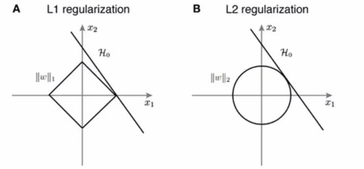
Shape of L1 and L2 Constraints

Geometrically, regularisation can be viewed as constraining weights to lie inside a norm ball.
For two parameters $(w_1, w_2)$ $(w_{1}, w_{2})$ :
- L1 constraint ( $|w_1| + |w_2| \le c$ ) forms a diamond.
- L2 constraint ( $w_1^2 + w_2^2 \le c$ ) forms a circle.
The sharp corners of the L1 diamond make it more likely to hit axes, producing exact zeros (sparsity).
The smooth L2 circle shrinks weights continuously, usually keeping them non-zero.

L1 vs L2 constraint geometry

L1 and L2 Regularisation In Practice

When to Use L1 and L2 Regularisation

When you need to reduce overfitting in linear models.
When features are correlated and coefficients are unstable (L2).
When you want automatic feature selection and sparsity (L1).
When training data is limited relative to feature count.

When Not to Use L1 and L2 Regularisation

When unshrunk coefficients are required for unbiased estimates.
When features are not standardised and penalties would be uneven.
When the true relationship is strongly nonlinear.
When constraints or priors already enforce complexity control.

Practical Notes

Preprocessing

Standardise all features before applying L1 or L2 penalties.

Model Selection

Tune $\lambda$ via cross-validation, not by training loss.
Use Elastic Net when you want sparsity with grouped features.

Interpretation

Track coefficient paths to understand shrinkage effects.