Syllabus Map

Study map: Syllabus Study Map

Overview

Clustering groups data by similarity without labels.
Different methods make different assumptions about cluster shape.

DBSCAN (Density-Based Spatial Clustering of Applications with Noise)

Core Idea

Groups points by density rather than distance alone.
Finds clusters of arbitrary shape.
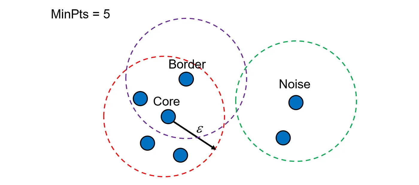
Classifies points as:
- Core points: have at least min_samples points within radius eps.
- Border points: are close to a core point but are not themselves core.
- Noise points: are not density-reachable from any core point.

How It Works (Step-by-Step)

Step 1: Define Neighborhood and Density Threshold

Choose eps and min_samples.
For each point $x_i$ , define its $\varepsilon$ -neighborhood:

N_\varepsilon(x_i)=\{x_j \mid d(x_i,x_j)\le \varepsilon\}

Step 2: Identify Core Points

A point is a core point if:

|N_\varepsilon(x_i)| \ge \text{min\_samples}

Points that are not core may later become border or noise points.

Step 3: Expand Clusters from Core Points

Start from an unvisited core point and create a new cluster.
Add all points that are density-reachable from it (directly or through a chain of core points).

Step 4: Attach Border Points

A border point is not core itself but lies in the $\varepsilon$ -neighborhood of a core point.
Border points are assigned to nearby expanded clusters.

Step 5: Label Remaining Points as Noise

Any point not assigned to a cluster is marked as noise (often label -1).

Key Hyperparameters

eps: neighborhood size. Too small can split clusters; too large can merge clusters.
min_samples: minimum local density. Higher values make the method more conservative.
metric: distance function (e.g., euclidean, manhattan, cosine).

Practical Notes

Handles outliers well.

Points that do not belong to dense regions are labeled as noise instead of being forced into a cluster.

Struggles with varying densities.

A single global eps may not fit both sparse and dense regions in the same dataset.

Scale features before DBSCAN.

DBSCAN is distance-based, so unscaled features can dominate neighborhood formation.

Hierarchical Clustering

Core Idea

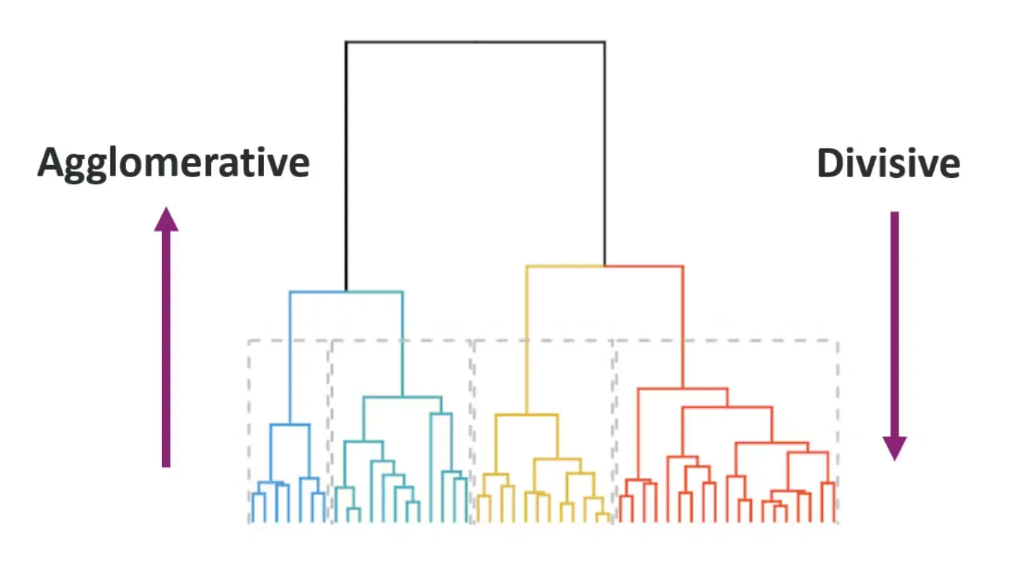
Builds a tree of clusters (dendrogram).
Can be agglomerative (bottom-up) or divisive (top-down).

How It Works (Step-by-Step)

Agglomerative Clustering (Bottom-Up)

Step 1: Compute Pairwise Distances

Build the distance matrix between data points:

d_{ij}=d(x_i,x_j)

Step 2: Initialise Singleton Clusters

Start with one cluster per point:

\mathcal{C}^{(0)}=\{\{x_1\},\{x_2\},\dots,\{x_n\}\}

Step 3: Measure Inter-Cluster Distance with a Linkage Rule

Linkage is the rule used to define the distance between two clusters $A$ and $B$ from point-level distances.
It determines which pair of clusters is considered “closest” and therefore merged next.
At each iteration, compute cluster distance using a chosen linkage (examples):
- Single linkage: $\min_{x\in A, y\in B} d(x,y)$
- Complete linkage: $\max_{x\in A, y\in B} d(x,y)$
- Average linkage: $\frac{1}{|A||B|}\sum_{x\in A,y\in B} d(x,y)$

Step 4: Merge Closest Clusters Iteratively

Merge the pair with minimum linkage distance.
Repeat until one cluster remains, recording merges to form a dendrogram.

Step 5: Cut the Dendrogram

Choose a cut height (or target number of clusters $k$ ).
Clusters below that cut become the final partition.

Divisive Clustering (Top-Down)

Step 1: Start with One Cluster

Place all points in a single cluster:

\mathcal{C}^{(0)}=\{\{x_1,x_2,\dots,x_n\}\}

Step 2: Select a Cluster to Split

Pick the cluster with highest heterogeneity (e.g., largest diameter or variance).
The goal is to split the least coherent cluster first.

Step 3: Split the Selected Cluster

Partition that cluster into two child clusters (often using a 2-way method such as k-means with $k=2$ ).
Choose the split that best improves within-cluster compactness and between-cluster separation.

Step 4: Repeat Recursive Splitting

Continue splitting clusters until a stopping rule is met.
Common stopping rules: target number of clusters, minimum cluster size, or low within-cluster variance.

Step 5: Read Final Clusters from the Dendrogram

The hierarchy can be cut at different levels to produce coarse or fine groupings.

Linkage Criteria

Single linkage: minimum pairwise distance between clusters.
Complete linkage: maximum pairwise distance between clusters.
Average linkage: average pairwise distance between clusters.
Ward linkage: merges that minimally increase within-cluster variance.

Practical Notes

No need to pre-specify number of clusters.

You can inspect the dendrogram first, then decide where to cut based on separation.

Can be expensive for large datasets.

Computing and storing pairwise distances can become costly in time and memory.

Choice of linkage changes cluster shape.

Different linkage rules can produce very different dendrograms on the same data.

Spectral Clustering

Core Idea

Uses eigenvectors of a graph Laplacian.
Finds clusters in a transformed space.

How It Works (Step-by-Step)

Step 1: Build an Affinity (Similarity) Matrix

Define similarity between points, for example with RBF kernel:

W_{ij}=\exp\left(-\frac{\|x_i-x_j\|^2}{2\sigma^2}\right)

Alternatively, use a k-NN graph to keep only local edges.

Step 2: Compute Degree Matrix and Graph Laplacian

Degree matrix:

D_{ii}=\sum_j W_{ij}

Unnormalised Laplacian:

L=D-W

Common normalised variant:

L_{\text{sym}}=I-D^{-1/2}WD^{-1/2}

Step 3: Solve Eigenproblem

Compute the first k eigenvectors of the chosen Laplacian.
Form embedding matrix $U\in\mathbb{R}^{n\times k}$ using these eigenvectors.

Step 4: Embed Points in Spectral Space

Represent each original point by its row in $U$ .
Nearby points in graph connectivity become closer in this transformed space.

Step 5: Cluster in the Embedded Space

Run k-means on rows of $U$ to produce final cluster labels.

Why It Helps

The spectral embedding separates points by graph connectivity.
This allows better recovery of non-convex clusters where plain k-means fails.

Practical Notes

Good for non-convex clusters.

Works well when clusters are connected components in a similarity graph rather than spherical blobs.

Requires choosing number of clusters.

You still need k (often selected via eigengap heuristics or validation).

Sensitive to graph construction.

Results depend on affinity choice (rbf, nearest_neighbors) and graph hyperparameters.

DBSCAN, Hierarchical & Spectral Clustering

Syllabus Map

Overview

DBSCAN (Density-Based Spatial Clustering of Applications with Noise)

Core Idea

How It Works (Step-by-Step)

Step 1: Define Neighborhood and Density Threshold

Step 2: Identify Core Points

Step 3: Expand Clusters from Core Points

Step 4: Attach Border Points

Step 5: Label Remaining Points as Noise

Key Hyperparameters

Practical Notes

Handles outliers well.

Struggles with varying densities.

Scale features before DBSCAN.

Hierarchical Clustering

Core Idea

How It Works (Step-by-Step)

Agglomerative Clustering (Bottom-Up)

Step 1: Compute Pairwise Distances

Step 2: Initialise Singleton Clusters

Step 3: Measure Inter-Cluster Distance with a Linkage Rule

Step 4: Merge Closest Clusters Iteratively

Step 5: Cut the Dendrogram

Divisive Clustering (Top-Down)

Step 1: Start with One Cluster

Step 2: Select a Cluster to Split

Step 3: Split the Selected Cluster

Step 4: Repeat Recursive Splitting

Step 5: Read Final Clusters from the Dendrogram

Linkage Criteria

Practical Notes

No need to pre-specify number of clusters.

Can be expensive for large datasets.

Choice of linkage changes cluster shape.

Spectral Clustering

Core Idea

How It Works (Step-by-Step)

Step 1: Build an Affinity (Similarity) Matrix

Step 2: Compute Degree Matrix and Graph Laplacian

Step 3: Solve Eigenproblem

Step 4: Embed Points in Spectral Space

Step 5: Cluster in the Embedded Space

Why It Helps

Practical Notes

Good for non-convex clusters.

Requires choosing number of clusters.

Sensitive to graph construction.